Download

1 / 23
230 likes | 328 Views
Warm-up. Get a sheet of computer paper/construction paper from the front of the room, and create your very own paper airplane. Try to create planes with different lengths from tip to end because we are going to test the length of a plane vs. distance travelled by the plane.

E N D
Warm-up • Get a sheet of computer paper/construction paper from the front of the room, and create your very own paper airplane. Try to create planes with different lengths from tip to end because we are going to test the length of a plane vs. distance travelled by the plane.
Cautions about Correlation and Regression and Section 3.3 Part of this is actually a section in Chapter 4!
Limitations of Correlation and Regression • They only describe LINEAR relationships. • They are NOT resistant to outliers or influential observations. • Always plot your data first!!!
The Question of Causation • This is a typical topic for AP Exam Questions!!! • Association does not imply causation. Did you know that ice cream sales and crime are positively correlated? i.e. As ice cream sales increase, so does the crime rate. Does that mean high ice cream sales CAUSE more crime? Well, let’s stop selling ice cream then! • Be careful: another variable may be at play here. As temperatures increase, ice cream sales increase. As temperatures increase, crime rate increases (people are simply more likely to be outside, so crime rates increase).
From Correlation to Regression • Regressionfinds the line that goes through the scatterplot and summarizes the relationship between the two variables. • Regression does require an explanatory and a response variable.
3.3 Least Squares Regression • If a scatterplot shows a linear trend, then we want to calculate a mathematical model for that data. This model will enable us to predict values based on the relationship between the two variables. • Called LSRL
Equations of Lines • In most math classes, the equation of a line is in the form y = mx + b. • Statisticians use the form • Notice that b is now the slope and a is the y-intercept!!! • Note: The LSRL ALWAYS goes through
On your Calculator • ALWAYS graph the data first! (use a scatterplot) • Ask yourself: is the data linear? • If it is not, linear regression is not appropriate! • If it is, press • STAT/CALC/8:LinReg L1, L2, Y1 (This automatically puts the equation into Y=). • Press GRAPH to see the line and the scatterplot together.
Calculating and using LSRL • Using the data from pg. 164, calculate the LSRL. • Estimate the weight gain if the NEA change is 300. • How did you find your estimate?
What does it all mean? • b, the slope represents the change in the expected y-value for every one x-value. • a, the y-intercept represents the predicted starting y-value.
Interpret the slope and y-intercept • A biologist wants to study the relationship between the number of trees x per acre and the number of birds y per acre. She came up with the equation of the regression line y = 5 + 4.2x
Reading Generic Computer Output The cell that represents the constant coefficient is the y-intercept. This will always say constant. The cell that represents the boat’s coefficient is the slope. It will give a variable name. So, my least-squares regression equation is
Extrapolation • Using the regression line for values far outside the domain of the explanatory variable. • Example: Let’s say we measure a child’s height every 6 months for the first 10 years of his/her life. While we may be able to predict the child’s height at age 11, predicting it at age 25 would not be accurate.
The Coefficient of Determination • r2, on the other hand, is the coefficient of determination. It tells us what percent of the variation in the response variable can be explained by the explanatory variable. • Fill in the blank sentence: r2 (%) of the variation in what y measures can be explain by what x measures. • Interpreting r2 = .721 if x is hours spent studying and y is GPA. • 72.1% of the variation in GPA can be explained by hours spent studying.
3.3 Residuals • A residual is the difference between what actual y value and the predicted y value. • Residual = observed y – predicted y • Residual = • When data points lie above the line, the residuals are positive. This means that the observed was higher than what the LSRL predicted. • The sum of the residuals = 0.
Example: Calculate the Residual • p. 234 Example 3.16. Type in the data. Then we will find the LSRL. • Child 1, who spoke at 15 months had an actual score of 95. What is their residual value? 2.0312
Residual Plots • A residual plot is a scatterplot of the observed explanatory variable vs the residuals.
To create a residual plot in your calculator… • In L3, type in L2 – Y1(L1). • This basically says you are going to take your actual y-values and subtract the predicted values… You have to plug in your x-values, which is where L1 comes from. • To see your plot, make a scatter plot of L1, L3.
Why Residuals are Important • Looking at a residual plots gives us an idea of whether the model we chose is appropriate. (Something may look like a line, but that may not be an appropriate model). • For any residual plot, a uniform scatter of points about the line (no obvious pattern) means that the data is a good fit for that model. • A residual plot that shows a curved pattern indicates that your choice of model is NOT a good fit. • If residuals are cone shaped, a your model is not a good fit. • The AP Exam notoriously shows residual plots for several different models and asks which model is best.
Is a line a good model? Bad Model!!! Good Model!
Outliers and Influential Observations • Outliers lie outside the overall pattern of the other observations. • These will be far above or below the other residuals on a residual plot.
Outliers and Influential Observations • Influential Observations markedly change the result of the calculation of the LSR line. Usually, points that are outliers in the x-direction of the scatterplot are influential.
Homework Chapter 3 #38, 40, 42, 54, 56