Download
1 / 36
360 likes | 438 Views
Learn about binomial distributions, Bernoulli trials, probability calculations, and applications in baseball and games.

E N D
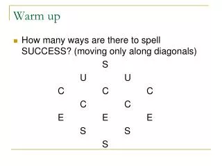
Warm up • How many ways are there to spell SUCCESS? (moving only along diagonals) S U U C C C C C E E E S S S
Warm up • How many ways are there to spell SUCCESS? S18 S9 S9 E3 E6 E3 C3 C3 C1 C2 C1 U1 U1 S1
Recall • A roulette wheel contains the following 38 numbers: • 0, 00, 1-36 (18 red, 18 black) • What is P(red)? • 18/38 = 0.47 • What is P(red,red)? • (18/38)2 = 0.22 • What is P(12 consecutive red)? • (18/38)12 = 0.000 13 • What is P(12 of 16 red)? • 0.018
5.3 Binomial Distributions Chapter 5.3 – Probability Distributions and Predictions Learning goal: Use Binomial Probabilities to calculate the probability of k successes in n trials Due now: 289 #1, 2aceg, 6-8, 11-12 MSIP/Home Learning: p. 299 #1, 3, 7, 8–12
Our Problem… • In any at-bat, a batter either gets a hit or he doesn’t (2 outcomes: success or failure) • Suppose his lifetime batting average is 0.292 • P(hit) = 0.292 in any at-bat • As the leadoff hitter he averages 5 AB per game • What are the possible outcomes for the number of hits he gets in 5 AB? • 0, 1, 2, 3, 4, 5 hits are possible • Are they all equally likely?
Binomial Experiments • Any experiment that has the following properties: • n identical trials • Two possible outcomes for each trial: success and failure • The probability of success is p • The probability of failure is 1 – p • The probabilities remain constant • The trials are independent • Bernoulli Trials - repeated independent trials with 2 possible outcomes (success and failure)
Bernoulli? • Jakob Bernoulli (Basel, Switzerland, December 27, 1654 - August 16, 1705) • Swiss Mathematician • One of the great names in probability theory
Binomial Distributions • In a binomial experiment: • The number of successes in n repeated Bernoulli Trials is a discrete random variable, X • X is termed a binomial random variable • Its probability distribution is called a binomial distribution • The following formula provides a method of solving complex probability problems…
Binomial Probability Distribution • Consider a binomial experiment in which there are n Bernoulli trials, each with a probability of success p • The probability of k successes in the n trials is given by:
Example 1a • Consider a game where a coin is flipped 5 times. You win the game if you get exactly 3 heads. What is the probability of winning? • We will let heads be a success • p = ½ • n = 5 • k = 3
Example 1b • Suppose the game is changed so that you win if you get at least 3 heads • what is the probability of winning now?
The Batting Example • the Expected Value of a binomial experiment that consists of n Bernoulli trials with a probability of success, p, on each trial is • E(X) = np • Example: Consider a baseball player who has a lifetime batting average of 0.292 • Let success be a hit where p = 0.292
a. What is the probability that he will get no hits in the next 5 at bats?
b. What is the probability that he gets 2 hits in the next 8 at bats?
c. What is the probability that he gets at least 1 hit in the next 10 at bats?
d. What is the expected number of hits in the next 10 at bats? • E(X) = np • E(X) = (10)(0.292) • = 2.92 ≈ 3 • therefore the player is expected to get 3 hits in the next 10 at bats
MSIP/ Home Learning • p. 299 #1, 3, 7, 8 – 12
Warm up • Describe a situation that could be represented by the following binomial probability: • It could be the probability that: • A 6 appears appears 5 times in 20 rolls of a standard die • A player who scores on 17% of his shots scores on 5 shots out of 20 • In a deck with the aces removed, a K or Q is drawn 5 times in 20 draws
Normal Approximation of the Binomial Distribution Chapter 5.4 – Probability Distributions and Predictions Learning Goal: Use the Normal Distribution to approximate Binomial Probabilities MSIP / Home Learning : p. 299 #1, 3, 7, 8 – 12 Fri MSIP / Home Learning: p. 311 # 4-10
Recall… • the probability of k successes in n trials (where p is the probability of success) is • this formula can only be used if we have a binomial distribution: • each trial is identical • the outcomes are either success or failure
This calculation is easy in simple cases… • Find the probability of 30 heads in 50 trials • So there is about a 4.2% chance • However, if we wanted to find the probability of tossing between 20 and 30 heads in 50 trials, we would need to perform 11 of these calculations • But…there is an easier way
Graphing the Binomial Distribution • If the distribution is approximately Normal, we can solve complex problems in the same way we did in the last chapter (z-Scores) • the question is: is the binomial distribution a normal one? • if the number of trials is sufficiently large, the binomial distribution approximates a normal curve
What does it look like? • when graphed the distribution of probabilities of heads looks like this • what will the mean be? • what will the standard deviation be?
So how do we work with all this • it turns out that a binomial distribution can be approximated by a normal distribution if: • np > 5 and n(1 – p) > 5 • if this is the case, the distribution is approximated by the normal distribution
But doesn’t a normal curve represent continuous data and a binomial distribution represent discrete data? • Yes! • So to use a normal approximation we have to consider a range of values rather than specific discrete values • Boundary values: • The interval for a value is from 0.5 below to 0.5 above, i.e., the interval for 10 goes from 9.5 to 10.5
Example 1 • Tossing a coin 50 times, what is the probability that you will get tails less than 20 times • let success be tails, so n = 50 and p = 0.5 • Test: • n x p = 50(0.5) = 25 > 5 • n x (1 - p) = 50(1 - 0.5) = 25 > 5 • now we can find the mean and the standard deviation
Example 1 continued • The boundary value is 19.5 • 20 is represented by the interval 19.5-20.5 • Less than 20 is actually less than 19.5 • z = 19.5 – 25 = -1.55 0.0606 • 3.54 • There is about a 6% chance of less than 20 tails in 50 attempts
In terms of the normal curve, it looks like this • all the values less than 19.5 are found in the shaded area 19.5 25.0
Example 2 • Two dice are rolled and the sum recorded 40 times. What is the probability that a sum greater than 6 occurs in over half of the trials? • let p be the probability of getting a sum greater than 6 • p = 6/36 + 5/36 + 4/36 + 3/36 + 2/36 + 1/36 = 7/12 • now we can do some calculations
Example 2 continued • the probability of getting a sum greater than 6 on more than half of the trials is 100 – 18 = 82%
Example 3 • you have a drawer with one blue mitten, one red mitten, one pink mitten and one green mitten • if you closed your eyes and picked a mitten at random 200 times (with replacement) what is the probability of choosing the pink mitten between 50 and 60 times (inclusive)? • so, success is considered to be drawing a pink mitten, with n = 200 and p = 0.25
Example 3 Continued • Test: • np = 200(0.25) = 50 > 5 • n(1 – p) = 200(0.75) = 150 > 5 • since both of these are greater than 5 the binomial distribution can be approximated by the normal curve • now find the mean and standard deviation
Example 3 Continued • the probability of having between 50 and 60 pink mittens (inclusive) drawn is 0.9564 – 0.4681 = 0.4883 or about 49%
MSIP/ Home Learning • Read the example on page 310 • do p. 311 # 4-10