Motivation
420 likes | 569 Views
Motivation. Histograms are everywhere in vision. object recognition / classification appearance-based tracking How do we compare two histograms {pi}, {qj}? Information theoretic measures like chi-square, Bhattacharyya coeff,

Motivation
E N D
Presentation Transcript
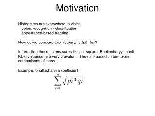
Motivation Histograms are everywhere in vision. object recognition / classification appearance-based tracking How do we compare two histograms {pi}, {qj}? Information theoretic measures like chi-square, Bhattacharyya coeff, KL-divergence, are very prevalent. They are based on bin-to-bin comparisons of mass. Example, bhattacharyya coefficient
problem is due to only considering intersection of mass in each bin. Not taking into account the ground-distance between nonoverlapping bins. = 0 for all pairs! Motivation Problem: the bin-to-bin comparison measures are sensitive to the binning of the data, and also to “shifts” of data acrossbins (say due to intensity gain/offset). Example, which of these is more similar to the black circle? 0 10 255 0 10 255 0 10 255 intensity intensity intensity
Earth Mover’s Distance ≠ example borrowed from Efros@cmu
The Difference? (amount moved) =
The Difference? (amount moved) * (distance moved) =
+X dist = xnew - xold Thought Experiment • move the books on your bookshelf one space to the right • you are lazy, so want to minimize sum of distances moved
strategy 1 strategy 2 Thought Experiment More than one minimal solution. Not unique! dist = 4 dist = 1 + 1 + 1 + 1 = 4
now minimize sum of squared distances Thought Experiment dist = 4^2 = 16 dist = 1^2+1^2+1^2+1^2 = 4 dist = 4 dist = 1 + 1 + 1 + 1 = 4 strategy 1 strategy 2
How Do We Know? How do we know those are the minimal solutions? Is that all of them? Let’s go back to abs distance |new-old| Form a table of distances |new-old| new A B C D E A 0 1 2 3 4 B 1 0 1 2 3 C 2 1 0 1 2 old D 3 2 1 0 1 A B C D E E 4 3 2 1 0
How Do We Know? How do we know those are the minimal solutions? Is that all of them? Let’s go back to abs distance |new-old| Form a table of distances |new-old| X off ones that are not admissable new A B C D E A x 1 2 3 4 B x 0 1 2 3 C x 1 0 1 2 old D x 2 1 0 1 A B C D E E x x x x x
How Do We Know? How do we know those are the minimal solutions? Is that all of them? Let’s go back to abs distance |new-old| Consider all permutations where there is asingle 1 in each admissable row and column. new A B C D E A x 1 2 3 4 B x 0 1 2 3 C x 1 0 1 2 old D x 2 1 0 1 A B C D E E x x x x x
How Do We Know? How do we know those are the minimal solutions? Is that all of them? Let’s go back to abs distance |new-old| Consider all permutations where there is asingle 1 in each admissable row and column. new A B C D E A x 1 2 3 4 B x 0 1 2 3 C x 1 0 1 2 old D x 2 1 0 1 A B C D E E x x x x x sum = 1+3+0+1 = 5
How Do We Know? How do we know those are the minimal solutions? Is that all of them? Let’s go back to abs distance |new-old| | Consider all permutations where there is asingle 1 in each admissable row and column. new A B C D E A x 1 2 3 4 B x 0 1 2 3 C x 1 0 1 2 old D x 2 1 0 1 A B C D E E x x x x x sum = 2+2+2+2 = 8
How Do We Know? How do we know those are the minimal solutions? Let’s go back to using absolute distance |new-old| Consider all permutations where there is asingle 1 in each admissable row and column. Try to find the minimum one! new A B C D E A x 1 2 3 4 B x 0 1 2 3 C x 1 0 1 2 old D x 2 1 0 1 A B C D E E x x x x x There are 4*3*2*1=24 permutations in this example. We can try them all. sum = 4+2+0+2 = 8
8 min solutions! It turns out that lot’s of solutions are minimal, when we use absolute distance.
How Do We Know? The two we had before are there. But there are others!! 4 1 2 3 1 2 3 4 3 1 2 4
now minimize sum of squared distances Recall: Thought Experiment dist = 4^2 = 16 dist = 1^2+1^2+1^2+1^2 = 4 dist = 4 dist = 1 + 1 + 1 + 1 = 4 strategy 1 strategy 2
new A B C D E A x 1 4 9 16 B x 0 1 4 9 C x 1 0 1 4 old D x 4 1 0 1 E x x x x x Only one unique min solution when we use |new-old|^2 This turns out to be the case for |new-old|^p for any p > 1 because then the cost function is strictly convex.
Other Ways to Look at It The way we’ve set it up so far, this problem is equivalent tothe linear assignment problem. We can therefore solve itusing the Hungarian algorithm.
Other Ways to Look at It We can also look at is as a min-costflow problem on a bipartite graph. (sources) (sinks) old position new position Instead of books, we canthink of these nodes asfactories and consumers, or whatever. Why? We can then think about relaxing the problemto consider fractional assignments between oldand new positions. (e.g. half of A goes to B, and the other half goes to C. cost(A,B) A B C D E A B C D E +1 -1 +1 -1 +1 -1 +1 -1 cost(D,E) more about this in a moment cost(old,new) = |new-old|^p
Mallow’s (Wasserstein) Distance X and Y be d-dimensional random variables. Prob distribution of X is P, and distribution of Y is Q. Also, consider some unknown distribution F overthe two of them taken jointly (X,Y) [dxd dimensional] Mallow’s distance: In words: Trying to find a minimum expected value of the distance between X and Y Expected value is taken over some unknown joint distribution F! F is constrained such that marginal wrt X is P, and marginal wrt Y is Q
Looking for set of values fij thatminimize sum new y1 y2 y3 y4 y5 P(xi) Subject to constraints: F has to be a prob distribution! *f11 *f31 *f21 *f41 *f51 *f52 *f32 *f12 *f22 *f42 *f43 *f23 *f33 *f53 *f13 *f24 *f14 *f44 *f54 *f34 *f25 *f55 *f35 *f45 *f15 x1 0 1 2 3 4 .25 x2 1 0 1 2 3 .25 x3 2 1 0 1 2 .25 old F has to have appropriate marginals x4 3 2 1 0 1 .25 x5 4 3 2 1 0 0 Q(yj) 0 .25 .25 .25 .25 Understanding Mallow’s Distance for discrete variables: costs dij
Mallow’s Versus EMD EMD Mallow’s For distributions they are the same. Also same when total masses are same
Mallow’s vs EMD main difference: EMD allows partial matches in the case of unequal masses. EMD = 0 Mallows = 1/2 note: using L1 norm As the paper points out, you have to be careful when allowing partial matches to make sure what you are doing is sensible.
Linear Programming Mallow’s/EMD for general d-dimensional data is solved vialinear programming, for example by the simplex algorithm. This makes it OK for low values of d (up to dozens), but makes it unsuitable for very large d. As a result, EMD is typically applied after clustering the data (say using k-means) into a smaller set of clusters. The coarse descriptors based on clusters are often called signatures.
Transportation Problem Mallow’s is a special case of linear programming : transportation problem formulated as a min-flow problem in a graph p1 -q1 p2 -q2 pm -qn
Assignment Problem some discrete cases (like our book example) simplify further : assignment problem formulated as a min-flow problem in a graph +1 -1 p1 -q1 +1 -1 p2 -q2 +1 -1 all x_ij are 0 or 1, and only one 1 in each row or column pm -qn
Linear Programming Mallow’s/EMD for general d-dimensional data is solved vialinear programming, for example by the simplex algorithm. This makes it OK for low values of d (up to dozens), but makes it unsuitable for very large d. As a result, EMD is typically applied after clustering the data (say using k-means) into a smaller set of clusters. The coarse descriptors based on clusters are often called signatures. However, If we use marginal distributions, so that we have 1D histograms,something wonderful happens!!!
(x) x F(x) 1 t 0 0 255 intensity (for example) One-Dimensional Data one dimensional data (like we’ve been using for illustration duringthis whole talk) is an important special case. Mallow’s/EMD distance computation greatly simplifies! First of all, for 1D, we can represent densities by their cumulativedistribution functions
One-Dimensional Data one dimensional data (like we’ve been using for illustration duringthis whole talk) is an important special case. Mallow’s/EMD distance computation greatly simplifies! First of all, for 1D, we can represent densities by their cumulativedistribution functions and the min distance can be computed as (x) x | F(x) – G(x) | dx
| F(x) – G(x) | dx One-Dimensional Data G(x) G-1(t) 1 1 F(x) F-1(t) t t 0 0 x x 0 255 0 255 intensity (for example) intensity (for example) just area between the two cumulative distribution function curves
Proof? It is easy to find papers that state the previous 1D simplified solution, but quite hard to find one with a proof! One is but you still have to work at it. I did, one week, and here is what I came up with: First, recall the quantile transform: given a cdf F(x), we can generate samples from it by uniformly sampling t ~ U(0,1) and then outputting F-1(t) F(x) 1 t0 ti ~ U(0,1) => xi ~ F t 0 x0 255 0 intensity (for example)
Proof? This allows us to understand that
consider an (abstract) example. Consider two density functions consider L2 cost function consider some (unknown) joint density Expected cost is sum ofthe 4x4 array of products. To compute Mallow’s distance, we want to choose pij to minimize this expected cost
-a +a +a -a Let min(p31,p14) = a > 0. now: subtract a from p31,p14 and add a to p11,p34 Note that the marginals have not changed! P.Major says: at minimum solution, for any pab and pcd on opposite sides ofthe diagonal, one or both of them should be zero. If not, we can construct alower cost solution. Example: our new cost differs from old on by –a(9+4) + a(0+1) = -12aso is a lower cost solution.
Connection (and a missing piece of the proof in P.Major’s paper) The above procedure serves to concentrate all the mass of the joint distribution along the diagonal, and apparently also yields the mincost solution.. However, concentration of mass along the diagonal is also a property of joint distributions of correlated random variables. Therefore... generating maximally correlated random variables via the quantile transformation should serve to generate a joint distribution clustered as tightly as possible around the diagonal of the cost matrix, and therefore, should yield the minimum expected cost. QED!!!!
Example: CDF Distance qj pi .25 .25 .25 .25 0 0 .25 .25 .25 .25 1 2 3 4 5 1 2 3 4 5 black = Pi = cdf of p white = Qi = cdf of q sum(Pi-Qi) = .25 + .25 + .25 + .25 + 0 = 1 Note: we get 1 instead of 4, the number we got earlier for the books,because we didn’t divide by total mass (4) earlier.
Example Application convert 3D color data into three 1D marginals compute CDF of marginal color data in a circular region compute CDF of marginal color data in a ring around that circle compare two CDFs using Mallow’s distance select peaks in the distance function as interest regions repeat, at a range of scales...