Download
1 / 24
240 likes | 376 Views
Define the methodologies to compare the resource indexing schemes Compare various resource indexing schemes. Motivation. Worst case number of bits per-allocation Calculate the worst case number of bits required for an allocation Commonly used metric For worst case design

E N D
Define the methodologies to compare the resource indexing schemes Compare various resource indexing schemes Motivation
Worst case number of bits per-allocation Calculate the worst case number of bits required for an allocation Commonly used metric For worst case design Ignores allocation pattern Ignores the size of allocation Worst case bit cost per-resource block allocated Calculate the worst case bit cost for one RB For worst case design Ignores allocation pattern Takes the size of allocation into consideration Average number of bits per-allocation Calculate the average number of bits required for an allocation assuming a particular allocation pattern For average performance design Take allocation pattern into consideration Ignores the size of allocation Average number of bits per-resource block allocated Calculate the average bit cost to allocate one resource block For average performance design Take allocation pattern into consideration Take the size of allocation into consideration Resource Indexing Metrics
Uniform distribution [RB_min, RB_max] The number of resource block allocated in each allocation is uniformly distributed over 1 RB (RB_min) and the maximum number of RBs (RB_max) Traffic dependent based on EVM traffic model Select packet size distribution based on traffic model in EVM (e.g. AMR 12.2 VoIP traffic model) Fixed MCS @ 1bits/sec/Hz or generate MCS distribution from SLS Calculate resource block allocation distribution from the packet size distribution and MCS distribution Allocation Pattern Modeling
Resource Allocation Evaluation Methodologies • Method 1: • Assume resource blocks are always contiguous in one allocation • Calculate the maximum number bits x(n) required of all possible allocations Hmax • Method 2: • Assume resource block are always contiguous in one allocation • Calculate the worst case bit cost for one RB • Method 3: • Assume resource block are always contiguous in one allocation • Assume allocated resource block size follow distribution P(n) • Assume required number of bits to index resource block size n is x(n) • Calculate the average number of bits required for one allocation • Method 4: • Assume resource block are always contiguous in one allocation • Assume allocated resource block size follow distribution P(n) • Assume required number of bits to index resource block size n is x(n) • Calculate the average number of bits required for one RB allocation
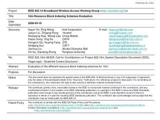
3GPP LTE Resource Allocation Approaches: Downlink • A resource allocation field in each PDCCH includes two parts, a type field and information consisting of the actual resource allocation. PDCCH with type 0 and type 1 resource allocation have the same format and are distinguished from each other via the type field. For system bandwidth less than or equal to 10 PRBs the resource allocation field in each PDCCH contains only information of the actual resource allocation. PDCCH with type 2 resource allocation have a different format from PDCCH with a type 0 or type 1 resource allocation. PDCCH with a type 2 resource allocation do not have a type field. • Resource Allocation Type 0 In resource allocations of type 0, a bitmap indicates the resource block groups that are allocated to the scheduled UE. The size of the group is a function of the system bandwidth that is shown: • Resource allocation type 0 is charaterized by the following: >> Grouping of RBs (in frequency domain): Group size may depend on system BW >> Bitmap indicates the RB groups to use At most 28 bits for 110 RB system BW At most 13 bits for 25 RB system BW >> Setting the limit on control signaling overhead.
3GPP LTE Resource Allocation Approaches: Downlink • Resource Allocation Type 1 In resource allocations of type 1, a bitmap indicates to a scheduled UE the resource blocks from the set of resource blocks from one of the P resource block group subsets where P is the resource block group size associated with the system bandwidth that is shown: • Resource Allocation Type 1 is characterized by the following: >> In this method, all resource blocks are divided into several sub-groups, wherein one example case dividing into two sub-groups is illustrated. >> The scheduler uses 1 sub-group to allocate resource to one UE. >> With this method, the number of signaling bits can be reduced because the scheduler uses one sub-group which consists of smaller number of RBs. The bitmap size can be expressed Nrb/m2, where m2 is the number of sub-groups.
3GPP LTE Resource Allocation Approaches: Downlink • Resource Allocation Type 2 In resource allocations of type 2, the resource allocation information indicates to a scheduled UE a set of contiguously allocated physical or virtual resource blocks depending on the setting of a 1-bit flag carried on the associated PDCCH. PRB allocations vary from a single PRB up to a maximum number of PRBs spanning the system bandwidth. For VRB allocations, the resource allocation information consists of a starting VRB number and a number of consecutive VRBs where each VRB is mapped to multiple non-consecutive PRBs. A type 2 resource allocation field consists of a resource indication value (RIV) corresponding to a starting resource block ( ) and a length in terms of contiguously allocated resource blocks ( ). The resource indication value is defined by: • Resource allocation type 2 is characterized by the following: >> In this method, the scheduler allocates resource with the unit of the island which consists of several contiguous RBs. The allocation information indicates the start point and the number of contiguous RBs. >> With this method, the number of signaling bits can be reduced because of compact expression thanks to contiguous RB allocation. However, when the number of islands is large, e.g., more than 2, the number of signaling bits becomes large. Also, it is a drawback that the number of signaling bits varies depending on the number of islands. It impacts on the receiver complexity in the UE. >> The signaling size for this allocation can be expressed , where m3 is the number of islands.
Option 1: Radix-2 Binary tree Option 2: Annular tree Option 3: Binary tree/bitmap hybrid Tree Based Allocation
Radix-2 Binary Tree • Bit overhead - Number of base nodes: N; - Number of Radix-2 based Nodes: - Number of Total Nodes based on the radix-2 tree: - Bit Overhead: ceil(log2(L)) • Bit Overhead of Radix-2-based Tree in case of N = 16.
Annular Tree • Annular Channel Tree Structure >> The base nodes are located on the outmost circle. The channel tree maintains a triangular structure for the outmost three levels and then switches to a power of two structure for the remaining levels. Such a structure results in a balance between the overhead associated with making time-frequency resource assignments and flexibility in the assignments. The levels of annular channel tree can be extended with the number of base nodes increasing. For the systems supporting the number of base nodes in the range of 2^n and 2^(n-1), n>2, the structures of annular channel tree are similar, except the number of null base nodes( null base node does not map to physical time-frequency resources). >> Bit overhead - Number of base nodes: N; - Number of Radix-2 based Nodes: - Number of Total Nodes based on the annular tree: - Bit Overhead ceil(log2(L))
Annular Tree Structure >> Take example - Number of base nodes: N = 32; - Number of Radix-2 based Nodes: M=25 = 32; - Number of Total Nodes based on the annular tree: L = 4M-1 = 4*32-1=127; - Bit Overhead for Option 1:log2(L) = log2(127) = 7bits
Annular Tree Indexing • Granularity of Continuous or Spaced Resource Blocks to be Allocated for Annular Channel Tree Structure
Annular Tree Indexing (cont’d) • Granularity of Continuous or Spaced Resource Blocks to be Allocated for Annular Channel Tree Structure is illustrated in case of N = 16.
Annular Tree Average Overhead • Average Bit Overhead of Continuous or Spaced Resource Blocks to be Allocated for Annular Channel Tree Structure is illustrated in case of N = 16.
Hybrid of a Power of Two Channel Tree and Bitmap Based Assignments >> The parent node is signaled using the power of two channel tree, while the child nodes are signaled using a bitmap, where each bit corresponds to one channel tree node. The delineation between the power of two signaling and the bitmap signaling is a system parameter, thereby making the assignment overhead flexible. >> Take example that the number of base nodes is 16 for allocations with bitmap indication. - Example 1: Parent Node 6 + bitmap ‘1000’ = base node 27 - Example 2: Parent Node 4 + bitmap ‘1110’ = base nodes 19, 20, 21 - Example 3: Parent Node 0 + bitmap ‘1100’ = channel tree nodes 3, 4 Tree/Bitmap Hybrid >> Bit Overhead [Which level of the child nodes is the bitmap indicated in relation to the parent nodes?] - Number of Base Nodes: N; - Number of Radix-2 Nodes: M = 2ceil(log2(N)); - System parameter delineating between the power of two signaling and bitmap signaling: ; - Bit Overhead for Option 2:
Tree/Bitmap Hybrid Indexing • Granularity of Continuous or Spaced Resource Blocks to be Allocated for Hybrid of a Power of Two Channel Tree and Bitmap Based Assignments [in case of N = 16]
Tree/Bitmap Hybrid Indexing (cont’d) • Granularity of Continuous or Spaced Resource Blocks to be Allocated for Hybrid of a Power of Two Channel Tree and Bitmap Based Assignments is illustrated [N = 16].
Tree/Bitmap Hybrid Average Overhead • Average Bit Overhead of Continuous or Spaced Resource Blocks to be Allocated for Hybrid of a Power of Two Channel Tree and Bitmap Based Assignments is illustrated in case of N = 16.
Uniformly Distributed Resource Allocation • Uniformly distributed resource allocation within [RB_min, RB_max] • Contiguous resource block for each allocation • Number of resource blocks=128 • *Note that LTE resource allocation type 0 and typ1 is not suitable for small packet size (e.g. VoIP) traffic due to the fact that the granularity of allocation for type 0 is 4RBs and that the granularity of allocation for type 1 is 1RB in case of the 20MHz (N = 128).
VoIP packet size: 44bytes (AMR 12.2) Resource block size: 12x6 Number of resource blocks: 128 MCS distribution generated from WiMAX SLS Contiguous resource allocation VoIP with MCS Distribution
MCS Distribution Sample MCS distribution from WiMAX SLS with mixed mobility (60% PB3, 30% VA30, 10% VA 120)
Overhead for VoIP Allocations • *Note that LTE resource allocation type 0 and typ1 is not suitable for small packet size (e.g. VoIP) traffic due to the fact that the granularity of allocation is 4RBs and that the granularity of allocation for type 1 is 1RB in case of the 20MHz (N = 128).
Worst case bit cost per allocation is not a good design criterion Average bit cost per allocation provides better measure of bit overhead for realistic traffic patterns Average/worst case bit cost per RB provides better measure of normalize bit overhead for each RB allocated Uniformly distributed allocation pattern is not a good pattern to evaluate the resource indexing overhead More realistic traffic model should be used Traffic model that is sensitive to resource indexing overhead (e.g. VoIP) should be used More accurate MCS level distribution model should provide better resource indexing overhead calculation Conclusions