Motivation

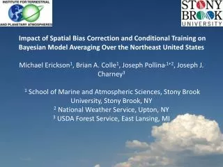
1. Impact of Spatial Bias Correction and Conditional Training on Bayesian Model Averaging Over the Northeast United StatesMichael Erickson1, Brian A. Colle1, Joseph Pollina,1+2, Joseph J. Charney31 School of Marine and Atmospheric Sciences, Stony Brook University, Stony Brook, NY2 National Weather Service, Upton, NY3 USDA Forest Service, East Lansing, MI

2. NCEP SREF Temperature Bias > 24oC Diurnal Mean Error – SREF/SBU 2X Bias • Ensembles have relatively large biases for commonly used surface variables (e.g. temperature, wind and precipitation). • Using the ensemble mean typically does not remove these biases. • Additionally, ensembles are underdispersed and not well calibrated even after bias correction. • Does the choice of bias correction matter, and does it vary with forecast variable? • How can post-processing be used to improve the forecasts associated with a particular flow regime (e.g. high fire threat days)? No Bias Motivation Questions to Be Addressed

3. Methods and Data • Analyzed the 18 to 42 hour forecasts from the Stony Brook University (SBU) and NCEP Short Range Ensemble Forecast (SREF) system for 2-m temperature and 10-m wind speed. • The Automated Surface Observing System (ASOS) are used as verifying observations from 2007-2009. Region of Study 00 UTC SBU 13 Member Ensemble • Consists of 7 MM5 and 6 WRF members run at 12 km grid spacing within a larger 36 km nest. • Variety of ICs (GFS, NAM, NOGAPS, CMC), microphysical, convective and PBL schemes. Verification Domain 21 UTC NCEP SREF 21 Member Ensemble • 10 ETA, 5 RSM, 3 WRF-NMM, and 3 WRF-ARW. • IC’s perturbed using a breeding technique.

4. Bias Correction Methods • Additive bias correction: Determine bias over training period and subtract it from forecast (Wilson et al. 2007): • Linear bias correction: Use linear regression with forecast model as the only predictor (Raftery et al. 2005 Wilson et al. 2007Sloughteret al. 2007, Sloughter et al. 2010). • CDF Bias Correction: Adjust the model CDF to the observed CDF for all forecast values (Hamill and Whitaker 2005), then elevation and landuse. • Additional Details • Training periods use the most recent 14 consecutive days. • Biases computed using a contigency table approach and averaged over models/hours. CDF Bias Correction Example CDF For Model and Observation

5. Linear Vs CDF Bias Correction – Warm Season 2007-2009 Temperature Bias by Threshold Wind Speed Bias by Threshold Wind Speed ETS by Threshold Temperature ETS by Threshold

6. Exploring Model Bias on Fire Threat Days Region of Study High Fire Threat Classification • Used the Fire Potential Index (FPI), and when not available the National Fire Danger Rating System (NFDRS), available through the Woodland Fire Assessment System (WFAS) from 2007-2009. • A Fire threat day must have 10% or greater of the domain reach 50 FPI or a NFDRS category of high. • Explored the impact of training period on post-processing for 86 fire threat days: • Sequential Training – Used the most recent 14 consecutive days. • Conditional Training – Used the most recent 5 fire threat days. • Wind speed bias corrected with the CDF method, temperature used the additive method.

7. Comparison of Sequential and Conditional Bias Correction for Fire Threat Days - Temperature Impact of Sequential Bias Correction - Temperature Conditional Vs Sequential Bias Correction For Fire Threat Days - Temperature

8. Comparison of Sequential and Conditional Bias Correction for Fire Threat Days – Wind Speed Impact of Sequential Bias Correction – Wind Speed Conditional Vs Sequential Bias Correction For Fire Threat Days – Wind Speed

9. Bayesian Model Averaging (BMA) • Bayesian Model Averaging (BMA, Raftery et al. 2005) calibrates ensemble forecasts by estimating: • Weights for each ensemble member. • The uncertainty associated with each forecast. • 10 members were selected from the SBU/SREF system (5 from MM5/WRF, 5 from the each of the SREF cores) with a training period of 50 days. • Parameters estimated using a MCMC method developed by Vrugt et al. (2008). The BMA derived distribution The coldest member is given the greatest weight The warmer members have varying weights The second coldest member is given significantly less weight From Raftery et al. 2005

10. Average BMA weights Using Sequential and Conditional Training – Temperature and Wind Speed Conditional Training – Wind Speed Conditional Training - Temperature Sequential Training - Temperature Sequential Training – Wind Speed

11. Rank Histograms/Reliability for Fire Threat Days after Applying Sequential/Conditional BMA - Temperature Rank Histogram - Sequential Rank Histogram - Conditional Reliability > 293 K - Sequential Reliability > 293 K Conditional Bias Corrected Bias Corrected

12. Rank Histograms/Reliability for Fire Threat Days after Applying Sequential/Conditional BMA – Wind Speed Rank Histogram - Sequential Rank Histogram - Conditional Reliability > 3.5 m/s - Sequential Reliability > 3.5 m/s - Conditional Bias Corrected Bias Corrected

13. Brier Skill Scores – Probabilistic Benefit of BMA Using Sequential and Conditional Training. • Blue line shows the probabilistic improvement (BSS > 0) of sequential bias correction and BMA compared to just using sequential bias correction. • Green line compares conditional bias correction and BMA to sequential bias correction. • Therefore BMA can be improved probabilistically by using conditional training. BMA BSS For Temperature BMA BSS For Wind Speed

14. Conclusions • The CDF bias correction removes 10-m wind speed bias more effectively on average than the additive or linear techniques. Overall, an additive or CDF bias correction works best for 2-m temperature. • Fire threat days exhibit warmer model temperature biases and lower wind speed biases than the warm season average. Therefore, using similar days to bias correct high fire threat events (conditional training) is more effective than using the most recent consecutive (sequential training) days. • Furthermore, conditional training with BMA improves ensemble calibration when compared to sequential training. • Conditional post-processing may be a valuable tool to more effectively bias correct and calibrate an ensemble for extreme weather events.