Download
1 / 23
230 likes | 256 Views
Explore turbulence properties using Doppler lidar and surface fluxes, including boundary-layer cloud forecasts and humidity convergence. Learn about refractivity mapping and turbulence evaluation.

E N D
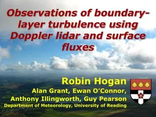
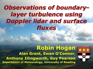
Observations of boundary-layer turbulence using Doppler lidar and surface fluxes Robin Hogan Alan Grant, Ewan O’Connor, Anthony Illingworth, Guy Pearson Department of Meteorology, University of Reading
Overview • Boundary-layer observations at Chilbolton • Boundary-layer height mapping (Cyril Morcrette) • Humidity convergence from refractivity (John Nicol) • Evaluation of boundary-layer cloud forecasts (Andrew Barrett) • Boundary-layer cloud microphysics (Ewan O’Connor) • Properties of turbulence from Doppler lidar and surface fluxes • Variance and skewness of vertical wind • The nature of turbulence driven by cloud-top radiative cooling • Potential for evaluating boundary layer parameterizations
Mapping BL top with radar Radar BL top Cyril Morcrette, MWR 2007 Radar sees clear-air scattering from refractive index inhomogeneities at boundary-layer top Mesoscale model BL top
Low-level atmospheric refractivity can be derived by measuring the phase shift between pieces of “ground clutter” with a scanning radar (higher refractivity usually means higher humidity) Refractivity • Animation of refractivity during the passage of a sea breeze from south: • Met Office working to assimilate it to provide information on humidity convergence as a precursor to convection John Nicol
Diurnal cycle composite of clouds Andrew Barrett, submitted to GRL Radar and lidar provide cloud boundaries and cloud properties above the site Meteo-France: Local mixing scheme: too little entrainment Swedish Met Institute: Prognostic TKE scheme: no diurnal evolution All other models have a non-local mixing scheme in unstable conditions and an explicit formulation for entrainment at cloud top: better performance over the diurnal cycle
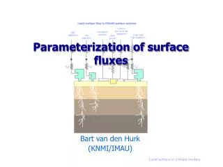
Fluxes on 11 July 2007 Most of incoming solar energy used for evaporation and transpiration Photosynthesis Turbulence
Input of sensible heat “grows” a new cumulus-capped boundary layer during the day (small amount of stratocumulus in early morning) Insects carried in updrafts to above the boundary layer top Convection is “switched off” when sensible heat flux goes negative at 1800 Surface heating leads to convectively generated turbulence
Comparing variance to previous studies • Lidar temporal resolution of ~30 s • Smallest eddies not detected, so add them using -5/3 law • Only valid in convective boundary layers where part of the inertial subrange is detected • Normalize variance by convective velocity scale • Reasonable agreement with Sorbjan (1980) and Lenschow et al. (1989) New contribution to variance
Skewness • Skewness defined as • Positive in convective daytime boundary layers • Agrees with aircraft observations of LeMone (1990) when plotted versus the fraction of distance into the boundary layer • Useful for diagnosing source of turbulence
Skewness in convective BLs • Both model simulations and laboratory visualisation show convective boundary layers heated from below to have narrow, intense updrafts and weak, broad downdrafts, i.e. positive skewness Narrow fast updrafts Wide slow downdrafts Courtesy Peter Sullivan NCAR
Why is skewness positive? • Consider TKE budget: • Vertical flux of TKE is • So skewness positive when TKE transported upwards by turbulence Stull TKE destroyed by dissipation & buoyancy suppression at BL top TKE transported upwards by turbulence TKE generated by shear and buoyancy in lower BL Transport
...a alternative related explanation • Updraft regions of large eddies have more intense small-scale turbulence than the downdraft regions • This leads to an asymmetric velocity distribution • Will test this later... Large eddies only All eddies
11 April 2007 Longwave cooling Positively buoyant plumes generated at surface: normal convection and positive skewness Cloud Negatively buoyant plumes generated at cloud top: upside-down convection and negative skewness Height Height Shortwave heating Potential temperature Potential temperature Stratocumulus cloud
Cospectrum Vertical wind from 11 April 2007 at time of transition • The cospectrum, Cww2: • Defined as the complex conjugate of FFT of w’ multiplied by FFT of w’ 2 • Can be thought of as a spectral decomposition of the third moment: • Hunt et al. (1988) showed that it goes as freq-2 in intertial subrange Skewness dominated by larger (20 minute timescale) eddies
Closed-cell stratocu. • Previous studies have shown updraft/downdraft asymmetry in stratocumulus at the largest scales • Puzzle as to why aspect ratio of cells is as much as 30:1 Shao & Randall (JAS 1996)
Comparison of top-down and bottom-up • Variance of vertical wind • Good agreement with previous studies if H = 30 W m-2 • Variance peaks in upper third of BL: agrees with Lenschow et al.’s fit provided theirs is inverted in height • Skewness • Very good agreement with the fit of LeMone (1990) to aircraft data provided hers is inverted in sign and height
Aircraft vs LES LES: Moeng and Wyngaard (1988) Aircraft observations: LeMone (1990)
Upside-down Carson’s model • If all the physics is the same but inverted, we can apply Carson’s model to predict the growth of the cloud-top-cooling driven mixed layer • With longwave cooling rate of H = 30 W m-2 and lapse rate of g = 1 K km-1, we estimate growth of 1.1 km in 3 hours, approximately the same as observed
Potential to evaluate the Lock BL scheme Very little turbulence Turbulence not reaching ground Negative skewness Lidar sees continuous cloud Turbulence throughout BL Skewness changes sign Lidar sees continuous cloud
Potential to evaluate the Lock BL scheme Turbulence with a minimum Skewness changes sign Lidar sees continuous cloud Turbulence with a minimum? Skewness of both signs Lidar sees Cu below Sc Turbulence below Cu base Negative skewness Lidar sees Cu
Conclusions • Many ways in which the Chilbolton instruments can be used to investigate the properties of the boundary layer • Variance and skewness from 2.5 years of continuous Doppler lidar data could be used to evaluate the categories predicted by the Lock boundary-layer scheme in the Met Office model • More details here: