Confounding and Interaction: Part III
770 likes | 1.03k Views
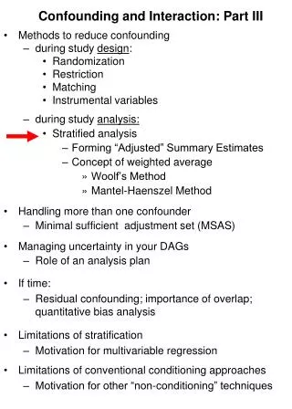
Confounding and Interaction: Part III. Methods to reduce confounding during study design : Randomization Restriction Matching Instrumental variables during study analysis: Stratified analysis Forming “Adjusted” Summary Estimates Concept of weighted average Woolf’s Method

Confounding and Interaction: Part III
E N D
Presentation Transcript
Confounding and Interaction: Part III • Methods to reduce confounding • during study design: • Randomization • Restriction • Matching • Instrumental variables • during study analysis: • Stratified analysis • Forming “Adjusted” Summary Estimates • Concept of weighted average • Woolf’s Method • Mantel-Haenszel Method • Handling more than one confounder • Minimal sufficient adjustment set (MSAS) • Managing uncertainty in your DAGs • Role of an analysis plan • If time: • Residual confounding; importance of overlap; quantitative bias analysis • Limitations of stratification • Motivation for multivariable regression • Limitations of conventional conditioning approaches • Motivation for other “non-conditioning” techniques
Effect-Measure Modification Crude RR crude= 1.7 Heavy Caffeine Use No Caffeine Use Stratified RRcaffeine use = 0.7 RRnocaffeine use = 2.4 . cs delayed smoking, by(caffeine) caffeine | RR [95% Conf. Interval] M-H Weight -----------------+------------------------------------------------- no caffeine | 2.414614 1.42165 4.10112 5.486943 heavy caffeine | .70163 .3493615 1.409099 8.156069 -----------------+------------------------------------------------- Crude | 1.699096 1.114485 2.590369 M-H combined | 1.390557 .9246598 2.091201 -----------------+------------------------------------------------- Test of homogeneity (M-H) chi2(1) = 7.866 Pr>chi2 = 0.0050 Report interaction; managing confounding by summarizing the 2 stratum-specific estimates into 1 number not relevant (but confounding is managed)
Report vs Ignore Effect-Measure Modification?Some Guidelines Is an art form: requires consideration of clinical, statistical and practical considerations P value threshold for reporting might be higher than other contexts, but interpretation is no different
Does AZT after needlesticks prevent HIV? Crude ORcrude = 0.61 Stratified Minor Severity Major Severity OR = 0.35 OR = 0.0
Ignore Interaction - B Report Interaction - A Need more information - C Does AZT after needlesticks prevent HIV? Report or ignore interaction?
Ignore Interaction - B Report Interaction - A Need more information - C Does AZT after needlesticks prevent HIV? Report or ignore interaction?
What Next? Crude ORcrude = 0.61 Stratified Minor Severity Major Severity OR = 0.0 OR = 0.35 How would you summarize these strata into one number?
Assuming Interaction is not Present, Form a Summary of the Unconfounded Stratum-Specific Estimates • Construct a weighted average • Assign weights to the individual strata • Summary Adjusted Estimate = Weighted Average of the stratum-specific estimates • a simple mean is a weighted average where the weights are equal to 1 • which weights to use depends on type of effect estimate desired (OR, RR, RD), characteristics of the data, and goal of research • e.g., • Woolf’s method • Mantel-Haenszel method • Standardization (see text) • Discussed earlier for age adjustment
Forming a Summary Adjusted Estimate for Stratified Data Crude ORcrude = 0.61 Stratified Minor Severity Major Severity OR = 0.0 OR = 0.35 How would you weight these strata? By number of cases - B Evenly - D By sample size - A By inverse of variance - E By degree of balance among cases/ controls - C
Forming a Summary Adjusted Estimate for Stratified Data Crude ORcrude = 0.61 Stratified Minor Severity Major Severity OR = 0.0 OR = 0.35 How would you weight these strata? By sample size - A By number of cases - B Evenly - D By inverse of variance - E By degree of balance among cases/ controls - C
Summary Estimators: Woolf’s Method • aka Directly pooled or precision estimator • Woolf’s estimate for adjusted odds ratio • where wi • wi is the inverse of the variance of the stratum-specific log(odds ratio)
Calculating a Summary Effect Using the Woolf Estimator • e.g., AZT use, severity of needlestick, and HIV Crude ORcrude =0.61 Stratified Minor Severity Major Severity OR = 0.0 OR = 0.35 Problem: cannot take log of 0; cannot divide by zero
Summary Adjusted Estimator: Woolf’s Method • Conceptually straightforward • Best when: • number of strata is small • sample size within each stratum is large • Cannot be calculated when any cell in any stratum is zero because log(0) is undefined • “1/2” cell corrections have been suggested but are subject to bias • Formulae for Woolf’s summary estimates for other measures (e.g., risk ratio, RD) available in texts and software documentation • Rarely used in practice but most clearly illustrates weighting
Summary Adjusted Estimators: Mantel-Haenszel • Mantel-Haenszel estimate for odds ratios • ORMH = • wi = • wi is inverse of the variance of the stratum-specific odds ratio under the null hypothesis (OR =1)
Summary Adjusted Estimator: Mantel-Haenszel • Relatively resistant to the effects of large numbers of strata with few observations • Resistant to cells with a value of “0” • Computationally easy • Bottomline: • Most commonly available technique in commercial software
Calculating a Summary Adjusted Effect Using the Mantel-Haenszel Estimator Crude • ORMH = • ORMH = ORcrude =0.61 Stratified Major Severity Minor Severity OR = 0.0 OR = 0.35
Calculating a Summary Effect in Stata • To stratify by a third variable: • cs varcase varexposed, by(varthird variable) • cc varcase varexposed, by(varthird variable) • Default summary estimator is Mantel-Haenszel • “ , pool” will also produce Woolf’s method • To stratify by several variables: • mhodds varcase varexposed varsadjust, by(var_liststratify) • Problem set this week • epitab command - Tables for epidemiologists • A good place to learn epidemiology
Calculating a Summary Effect Using the Mantel-Haenszel Estimator • e.g., AZT use, severity of needlestick, and HIV • . cc HIV AZTuse,by(severity) pool • severity | OR [95% Conf. Interval] M-H Weight • -----------------+------------------------------------------------- • minor | 0 0 2.302373 1.070588 • major | .35 .1344565 .9144599 6.956522 • -----------------+------------------------------------------------- • Crude | .6074729 .2638181 1.401432 • Pooled (direct) | . . . • M-H combined | .30332 .1158571 .7941072 • -----------------+------------------------------------------------- • Test of homogeneity (B-D) chi2(1) = 0.60 Pr>chi2 = 0.4400 • Test that combined OR = 1: • Mantel-Haenszel chi2(1) = 6.06 • Pr>chi2 = 0.0138 Crude ORcrude =0.61 Stratified Minor Severity Major Severity OR = 0.0 OR = 0.35
After the Point Estimate: Confidence Interval Estimation and Hypothesis Testing for the Mantel-Haenszel Estimator • e.g. AZT use, severity of needlestick, and HIV • . cc HIV AZTuse,by(severity) pool • severity | OR [95% Conf. Interval] M-H Weight • -----------------+------------------------------------------------- • minor | 0 0 2.302373 1.070588 • major | .35 .1344565 .9144599 6.956522 • -----------------+------------------------------------------------- • Crude | .6074729 .2638181 1.401432 • Pooled (direct) | . . . M-H combined | .30332 .1158571 .7941072 • -----------------+------------------------------------------------- • Test of homogeneity (B-D) chi2(1) = 0.60 Pr>chi2 = 0.4400 • Test that combined OR = 1: • Mantel-Haenszel chi2(1) = 6.06 • Pr>chi2 = 0.0138 • ?
After Confounding is Managed: Confidence Interval Estimation and Hypothesis Testing for the Mantel-Haenszel Estimator • e.g. AZT use, severity of needlestick, and HIV • . cc HIV AZTuse,by(severity) pool • severity | OR [95% Conf. Interval] M-H Weight • -----------------+------------------------------------------------- • minor | 0 0 2.302373 1.070588 • major | .35 .1344565 .9144599 6.956522 • -----------------+------------------------------------------------- • Crude | .6074729 .2638181 1.401432 • Pooled (direct) | . . . M-H combined | .30332 .1158571 .7941072 • -----------------+------------------------------------------------- • Test of homogeneity (B-D) chi2(1) = 0.60 Pr>chi2 = 0.4400 • Test that combined OR = 1: • Mantel-Haenszel chi2(1) = 6.06 • Pr>chi2 = 0.0138 • What does the p value = 0.0138 mean? If there truly is no association between azt and HIV acquisition after adjustment for severity of exposure, there is a 1.38% probability of obtaining an OR of 0.30 or more extreme by chance alone. - C 1.38% probability that the adjusted OR = 0.30 is due to chance - A 1.38% probability that the difference between crude and adjusted OR is due to chance - B Some better answer - D
After Confounding is Managed: Confidence Interval Estimation and Hypothesis Testing for the Mantel-Haenszel Estimator • e.g. AZT use, severity of needlestick, and HIV • . cc HIV AZTuse,by(severity) pool • severity | OR [95% Conf. Interval] M-H Weight • -----------------+------------------------------------------------- • minor | 0 0 2.302373 1.070588 • major | .35 .1344565 .9144599 6.956522 • -----------------+------------------------------------------------- • Crude | .6074729 .2638181 1.401432 • Pooled (direct) | . . . M-H combined | .30332 .1158571 .7941072 • -----------------+------------------------------------------------- • Test of homogeneity (B-D) chi2(1) = 0.60 Pr>chi2 = 0.4400 • Test that combined OR = 1: • Mantel-Haenszel chi2(1) = 6.06 • Pr>chi2 = 0.0138 • What does the p value = 0.0138 mean? If there truly is no association between azt and HIV acquisition after adjustment for severity of exposure, there is a 1.38% probability of obtaining an OR of 0.30 or more extreme by chance alone. - C 1.38% probability that the adjusted OR = 0.30 is due to chance - A 1.38% probability that the difference between crude and adjusted OR is due to chance - B Some better answer - D
Terminology • “Use of AZT is associated with decreased odds of HIV acquisition, independent of needlestick severity” • “Use of AZT is associated with decreased odds of HIV acquisition, adjusted for needlestick severity” • “Use of AZT is associated with decreased odds of HIV acquisition, controlling for needlestick severity” • “Use of AZT is associated with decreased odds of HIV acquisition, conditioned on needlestick severity”
“Independent of” • “Use of AZT is associated with decreased odds of HIV acquisition, independent of needlestick severity” • “independent of” simply refers to adjustment/control for specific factors • Does not refer to whether or not adjusted estimate is different from crude • Just means that adjustment has been performed (e.g., via stratification)
How about this? • “Use of AZT is causally related to reduced HIV acquisition.” • Formally, our analyses produce statistical associations, which could result from: • Causal relationship (Truth) • Or bias due to: • Selection bias • Measurement bias • Confounding bias • Or • Reverse causality (but not here since we know AZT use came first) • Or • Chance • Single observational study rarely proves causality • Data themselves do not establish causality • - Scientists do, by consensus, by excluding the other 5 explanations
Mantel-Haenszel Techniques • Mantel-Haenszel estimators • Mantel-Haenszel chi-square statistic • Mantel’s test for trend (dose-response)
Smoking Age CAD Chlamydia pneumoniaeinfection ? More than One Confounder RQ: Does Chlamydia pneumoniae infection cause coronary artery disease (CAD)?
Stratifying by Multiple Confounders Confounders:Age and Smoking • To control for multiple confounders simultaneously, must construct mutually exclusive and exhaustive strata:
Because Confounders Operate Together in Nature, Joint Stratification is Needed Crude Stratified <40 smokers 40-60 smokers >60 smokers <40 non-smokers 40-60 non-smokers >60 non-smokers Next steps: Assess for interaction… summarize….
WHO Causal Model of Coronary Heart Disease Murray et al. Population Health Metrics 2003
Minimal Sufficient Adjustment Sets(MSAS) • Minimal set of variables, which if controlled for, will allow for estimation of causal effect of E on D • i.e., the minimal set of factors you need to control for that will: • keep all causal paths open • and • close all non-causal paths • Remember, the general statistical term for “controlled for” is “condition” • means to hold constant • techniques include: restriction, matching, stratification, or mathematical regression • For any DAG, there may be several minimal sufficient adjustment sets (MSAS’s).
Real life DAGs make it very difficult for the human eye to manually determine the MSAS’s • DAGitty.net makes it simple
Why might we decide to adjust for one MSAS over another? • Not all variables are created equal • i.e., not all variables are equally easy to control for • Some variables: • Have lots of missing data • Are poorly measured • Either reproducibility or validiity • Difficult to quantity • e.g., injection drug use, or hypertension • Difficult to specify • e.g., continuous variables • Expensive to measure • Involve ethical issues if measured • e.g., illegal behavior (drug use; commercial sex) • Advice • Choose MSAS which has variables that are most feasible, reproducible, accurate, and manageable
Need h in all scenarios If k is a problem to measure, go for {a, h, i}
B ? A ? D E ? The Ideal You are confident about the DAG • Find all the MSASs • Choose the most practical MSAS • Adjust for the chosen MSAS • Via restriction, matching, stratification, or regression • Report the final adjusted measure of association The Reality You are often NOT confident about the DAG • Why not just take the most conservative route and adjust for everything that is conceivable?
Crude ORcrude = 21.0 (95% CI: 16.4 - 26.9) Matches Present Matches Absent Stratified ORmatches = 21.0 OR nomatches = 21.0 ORadj MH= 21.0 (95% CI: 14.2 - 31.1) Which will you report as your final answer? Adjusted - B Crude - A Need more information- C
Crude ORcrude = 21.0 (95% CI: 16.4 - 26.9) Matches Present Matches Absent Stratified ORmatches = 21.0 OR nomatches = 21.0 ORadj MH= 21.0 (95% CI: 14.2 - 31.1) Which will you report as your final answer? Crude - A Adjusted - B Need more information- C
No indication from the DAG that Matches must be controlled for Matches Lung Cancer Smoking ?
Effect of Adjustment on Precision (Variance) • Adjustment (e.g., stratification) is not all good • Adjustment can increase or decrease standard errors (and CI’s) depending upon: • Nature of outcome (interval scale vs. binary) • Measure of association desired • Method of adjustment (Woolf vs M-H vs MLE) • Strength of association between potential confounding factor and exposure/disease • Difficult to predict effect on precision • Good news: adjustment for strong confounders removes bias and often improves precision • Bad news: adjustment for less-than-strong confounders can often (but not always) worsen precision
Spermicides, maternal age & Down Syndrome Crude OR = 3.5 Age < 35 Age > 35 Stratified OR = 3.4 OR = 5.7 Which answer should you report as “final”? Adjusted - B Crude - A Need more information- C
Spermicides, maternal age & Down Syndrome Crude OR = 3.5 Age < 35 Age > 35 Stratified OR = 3.4 OR = 5.7 Which answer should you report as “final”? Crude - A Adjusted - B Need more information- C
What if you don’t know if the red edge exists? (i.e., existing literature is inconclusive) Age ? Down Syndrome Spermicide use ?
Whether or not to accept the “adjusted” summary estimate instead of the crude? • No one correct answer • “Bias-variance tradeoff” • Scientifically rigorous approach is to: • Create the DAG and identify potential confounders • Prior to adjustment, classify the potential confounders as either being: • “A” List: Those factors for which you will accept the adjusted result no matter how small the difference from the crude. • Factors strongly believed to be confounders • “B” List: Those factors for which you will accept the adjusted result only if it meaningfully differs from the crude (with some pre-specified difference, e.g., 5 to 10%). • Factors you are less sure about • “Change-in-estimate” approach • For some analyses, may have no factors on B list. For other analyses, some factors on B list. • Always putting all factors on A list may seem “conservative”, but not necessarily the right thing to do in light of penalty of statistical imprecision Bias control paramount Need for tradeoffs
Adjusting for Age? Age is on “A” List Adjust for Age; Accept OR = 3.8 as final estimate Age Age Down Syndrome Down Syndrome Spermicide use ? ? Whether age is on “A” or “B” list should be pre-specified in your analysis plan Age is on “B” List Adjust for Age only if exceeds pre-specified change-in- estimate threshold (e.g., 10%) ? Spermicide use
Choosing the crude or adjusted estimate? • Assume no interaction • Factors on B list have 10% change-in-estimate rule in place
“Change in Estimate” Approach– A Historical Perspective • Historically, confounding was defined by whether the adjusted estimate differed from the crude • “if there is a change after adjustment, there has to be confounding present” • i.e., in the past, the data defined confounding • “data-based definition of confounding” • Today, philosophy is very different • We primarily don’t use data from the current study to define presence or absence confounding or what to control for • e.g., if we adjust for something and it changes the estimate, we don’t accept this as confounding unless there was some a priori belief (e.g., gum chewing in melonoma) • Exception: if the prior literature is uncertain about a part of a DAG, it is reasonable to use data from current study to weigh in on the decision to adjust • This is the “change in estimate” approach
No Role for Statistical Testing for Confounding • Testing for statistically significant differences between crude and adjusted measures is inappropriate • e.g., examining an association for which a factor is a known confounder (say age in the association between hypertension and CAD) • if the study has a small sample size, even large differences between crude and adjusted measures may not be statistically different • yet, we know confounding is present • therefore, the difference between crude and adjusted measures cannot be ignored as merely chance. • bias must be prevented and hence adjusted estimate is preferred • we must live with whatever effects we see after adjustment for a factor for which there is a strong a priori belief about confounding • If study has large sample size, even small differences between crude and adjusted will be significant. Would you accept all of these adjustments to be necessary even if no a priori evidence of confounding?
The Ideal You are confident about the DAG • Find all the MSASs • Choose the most practical MSAS • Adjust for the chosen MSAS • Via restriction, matching, stratification, or regression • Report the final adjusted measure of association The Reality You are often NOT confident about the DAG • Why not just take the most conservative route and adjust for everything that is conceivable? • Problems with this approach: • Precision (increase variance) • Bias (if inadvertent adjustment on a collider)