Self-Organizing Map (SOM)
Self-Organizing Map (SOM). Unsupervised neural networks, equivalent to clustering. Two layers – input and output The input layer represents the input variables. The output layer: neurons arranged in a single line (one-dimensional) or a two-dimensional grid. Main feature – weights.

Self-Organizing Map (SOM)
E N D
Presentation Transcript
Unsupervised neural networks, equivalent to clustering. • Two layers – input and output • The input layer represents the input variables. • The output layer: neurons arranged in a single line (one-dimensional) or a two-dimensional grid. • Main feature – weights
Learning means adopting the weights. • Each output receives inputs through the weights. weight vector has the same dimensionality as the input vector • The output of each neuron is its activation – weighted sum of inputs (i.e. linear activation function). u = x1w11 + x2w21 w21 w11 2
The objective of learning: project high-dimensional data onto 1D or 2D output neurons. • Each neuron incrementally learns to represent a cluster of data. • The weights are adjusted incrementally – the weights of neurons are called codebook vectors (codebooks).
Competitive learning • The so-called competitive learning(winner-takes-all) . • Competitive learning will be demonstrated on simple 1D network with two inputs. Sandhya Samarasinghe, Neural Networks for Applied Sciences and Engineering, 2006
First, number of output neurons (i.e. clusters) must be selected. • Not always known, do reasonable estimate, it is better to use more, not used neurons can be eliminated later. • Then initialize weights. • e.g., small random values • Or randomly choose some input vectors and use their values for the weights. • Then competitive learning can begin.
The activation for each output neuron is calculated as weighted sum of inputs. • e.g., the activation of the output neuron 1 is u1 = w11x1 + w21x2. Generally • Activation is the dot product between input vector x and weight vector wj. Sandhya Samarasinghe, Neural Networks for Applied Sciences and Engineering, 2006
Dot product is not only , but also • If |x| = |wj| = 1, then uj = cosθ. • The closer these two vectors are (i.e. the smaller θ is), the bigger the uj is (cos 0 = 1). x w θ
Say it again, and loudly: The closer the weight and input vectors are, the bigger the neuron activation is. Dan na Hrad. • A simple measure of the closeness – Euclidean distance between x and wj.
Scale the input vector so that its length is equal to one. |x|=1 • An input is presented to the network. • Scale weight vectors of individual output neurons to the unit length. |w|=1 • Calculate, how close the input vector xis to each weight vector wj (j is 1 … # output neurons). • The neuron which codebook is closest to the input vector becomes a winner (BMU, Best Matching Unit). • Its weights will be updated.
Weight update • The weight vector w is updated so that it moves closer to the input x. d x Δw β – learning rate w
Recursive vs. batch learning • Conceptually similar to online/batch learning • Recursive learning: • update weights of the winning neuron after each presentation of input vector • Batch learning: • note the weight update for each input vector • the average weight adjustment for each output neuron is done after the whole epoch • When to terminate learning? • mean distance between neurons and inputs they represent is at a minimum, distance stops changing
Example Sandhya Samarasinghe, Neural Networks for Applied Sciences and Engineering, 2006
Sandhya Samarasinghe, Neural Networks for Applied Sciences and Engineering, 2006
epoch Sandhya Samarasinghe, Neural Networks for Applied Sciences and Engineering, 2006
Sandhya Samarasinghe, Neural Networks for Applied Sciences and Engineering, 2006
Sandhya Samarasinghe, Neural Networks for Applied Sciences and Engineering, 2006
Topology is not preserved. Sandhya Samarasinghe, Neural Networks for Applied Sciences and Engineering, 2006
Meet today’s hero Teuvo Kohonen
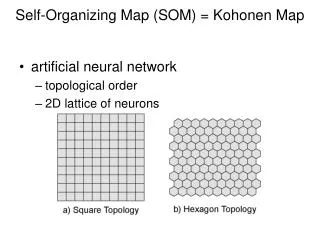
Self-Organizing Maps • SOM, also Self-Organizing Feature Map (SOFM), Kohonen neural network. • Inspired by the function of brain: • Different brain regions correspond to specific aspects of human activities. • These regions are organized such that tasks of similar nature (e.g. speech and vision) are controlled by regions that are in spatial proximity each to other. • This is called topology preservation.
In SOM learning, not only the winner, but also the neighboring neurons adapt their weights. • Neurons closer to the winner adjust weights more than further neurons. • Thus we need • to define the neighborhood • to define a way how much neighboring neurons adapt their weights
Neighborhood definition neighborhood radius r 2 1 1 1 2 2 1 3 2 Sandhya Samarasinghe, Neural Networks for Applied Sciences and Engineering, 2006
Training in SOM • Follows similar manner of standard winner-takes-all competitive training. • However, new rule is used for weight changes. • Suppose, that the BMU is at position {iwin, jwin} on the 2D map. • Then all codebook vectors of BMU and neighbors are adjusted to w’j according to where NS is the neighbor strength varying with the distance to the BMU. β is learning rate.
Neighbor strength • When using neighbor features, all neighbor codebooks are shifted towards the input vector. • However, BMU updates most, and the further away the neighbor neuron is, the less its weights update. • The NS function tells us how the weight adjustment decays with distance from the winner.
Gaussian Linear Sandhya Samarasinghe, Neural Networks for Applied Sciences and Engineering, 2006 Exponential
2D Side Effects source: http://www.cis.hut.fi/projects/somtoolbox/download/sc_shots2.shtml
Shrinking neighborhood size • Large neighborhood – proper placement of neurons in the initial stage to broadly represent spatial organization of input data. • Further refinement – subsequent shrinking of the neighborhood. • A size of large starting neighborhood is reduced with iterations. σ0 … initial neighborhood size σt … neighborhood size at iteration t T … total number of iterations bringing neighborhood to zero (i.e., only winner remains) linear decay exponential decay
Learning rate decay • The step length (learning rate ) is also reduce with iterations. • Two common forms: linear or exponential decay • Strategy: start with relatively high β, decrease gradually, but remain above 0.01 … constant bringing to zero (or small value) Weight update incorporating learning rate and neighborhood decay
Recursive/Batch Learning • SOM in a batch mode with no neigborhood is equivalent to k-means • The use of neighborhood leads to topology preservation • Regions closer in input space are represented by neurons closer in a map.
Two Phases of SOM Training • Two phases • ordering • convergence • Ordering • neighborhood and learning rate are reduced to small values • topological ordering • starting high, gradually decrease, remain above 0.01 • neighborhood – cover whole output layer • Convergence • fine tuning with the shrunk neighborhood • small non-zero (~0.01) learning rate, NS no more than 1st neighborghood
Example contd. Sandhya Samarasinghe, Neural Networks for Applied Sciences and Engineering, 2006
Sandhya Samarasinghe, Neural Networks for Applied Sciences and Engineering, 2006 neighborhood drops to 0 after 3 iterations
After 3 iterations topology preservation takes effect very quickly Complete training Converged after 40 epochs. Epochs Sandhya Samarasinghe, Neural Networks for Applied Sciences and Engineering, 2006
Complete training • All vectors have found cluster centers • Except one • Solution: add one more neuron 4 3 5 6 2 1 Sandhya Samarasinghe, Neural Networks for Applied Sciences and Engineering, 2006
4 3 5 6 2 7 1 Sandhya Samarasinghe, Neural Networks for Applied Sciences and Engineering, 2006
2D output • Play with http://www.demogng.de/ • Choose 'The self-organizing map'. Following update formulas are used: neighborhood size learning rate
A self-organizing feature map from a square source space to a square (grid) target space. Duda, Hart, Stork, Pattern Classification, 2000
Some initial (random) weights and the particular sequence of patterns (randomly chosen) lead to kinks in the map; even extensive further training does not eliminate the kink. In such cases, learning should be restarted with randomized weights and possibly a wider window function and slower decay in learning. Duda, Hart, Stork, Pattern Classification, 2000
2D maps of multidimensional data • Iris data set • 150 patterns, 4 attributes, 3 classes (Setosa – 1, Versicolor – 2, Virginica – 3) • more than 2 dimensions, so all data can not be vizualized in a meaningful way • SOM can be used not only to cluster input data, but also to explore the relationships between different attributes. • SOM structure • 8x8, hexagonal, exp decay of learning rate β (βinit = 0.5, Tmax = 20x150 = 3000), NS: Gaussian
virginica versicolor setosa • What can be learned? • petal length and width have structure similar to the class panel • low length correlates with low width and these relate to the Versicolor class • sepal width – very different pattern • class panel – boundary between Virginica and Setosa – classes overlap Sandhya Samarasinghe, Neural Networks for Applied Sciences and Engineering, 2006
Since we have class labels, we can assess the classification accuracy of the map. • So first we train the map using all 150 patterns. • And then we present input patterns individually again and note the winning neuron. • The class to which the input belongs is the class associated with this BMU codebook vector (see previous slide, Class panel). • Only the winner decides classification.
Only winner decides the classification Vers (2) – 100% accuracy Set (1) – 86% Virg (3) – 88% Overall accuracy = 91.3% Neighborhood of size 2 decides the classification Vers (2) – 100% accuracy Set (1) – 90% Virg (3) – 94% Overall accuracy = 94.7% Sandhya Samarasinghe, Neural Networks for Applied Sciences and Engineering, 2006