Self-Organizing Maps: A Comprehensive Guide
260 likes | 389 Views
Explore the biological motivation, architecture, and examples of SOMs, a special case of competitive learning crucial in data analysis and feature extraction.

Self-Organizing Maps: A Comprehensive Guide
E N D
Presentation Transcript
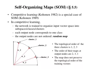
Self-Organizing Maps (SOM) (§ 5.5) • Competitive learning (Kohonen 1982) is a special case of SOM (Kohonen 1989) • In competitive learning, • the network is trained to organize input vector space into subspaces/classes/clusters • each output node corresponds to one class • the output nodes are not ordered: random map cluster_1 • The topological order of the three clusters is 1, 2, 3 • The order of their maps at output nodes are 2, 3, 1 • The map does not preserve the topological order of the training vectors cluster_2 w_2 w_3 cluster_3 w_1
Topographic map • a mapping that preserves neighborhood relations between input vectors, (topology preserving or feature preserving). • if are two neighboring input vectors ( by some distance metrics), • their corresponding winning output nodes (classes), i and j must also be close to each other in some fashion • one dimensional: line or ring, node i has neighbors or • two dimensional: grid. rectangular: node(i, j) has neighbors: hexagonal: 6 neighbors
Biological motivation • Mapping two dimensional continuous inputs from sensory organ (eyes, ears, skin, etc) to two dimensional discrete outputs in the nerve system. • Retinotopic map: from eye (retina) to the visual cortex. • Tonotopic map: from the ear to the auditory cortex • These maps preserve topographic orders of input. • Biological evidence shows that the connections in these maps are not entirely “pre-programmed” or “pre-wired” at birth. Learning must occur after the birth to create the necessary connections for appropriate topographic mapping.
SOM Architecture • Two layer network: • Output layer: • Each node represents a class (of inputs) • Neighborhood relation is defined over these nodes • Nj(t): set of nodes within distance D(t) to node j. • Each node cooperates with all its neighbors and competes with all other output nodes. • Cooperation and competition of these nodes can be realized by Mexican Hat model D = 0: all nodes are competitors (no cooperative) random map D > 0: topology preserving map
Notes • Initial weights: small random value from (-e, e) • Reduction of : Linear: Geometric: • Reduction of D: should be much slower than reduction. D can be a constant through out the learning. • Effect of learning For each input i, not only the weight vector of winner is pulled closer to i, but also the weights of ’s close neighbors (within the radius of D). • Eventually, becomes close (similar) to . The classes they represent are also similar. • May need large initial D in order to establish topological order of all nodes
Notes • Find j* for a given input il: • With minimum distance between wj and il. • Distance: • Minimizing dist(wj, il) can be realized by maximizing
Examples • A simple example of competitive learning (pp. 172-175) • 6 vectors of dimension 3 in 3 classes, node ordering: B – A – C • Initialization: , weight matrix: • D(t) = 1 for the first epoch, = 0 afterwards • Training with • determine winner: squared Euclidean distance between • C wins, since D(t) = 1, weights of node C and its neighbor A are updated, bit not wB
Examples • Observations: • Distance between weights of non-neighboring nodes (B, C) increase • Input vectors switch allegiance between nodes, especially in the early stage of training
How to illustrate Kohonen map (for 2 dimensional patterns) • Input vector: 2 dimensional Output vector: 1 dimensional line/ring or 2 dimensional grid. Weight vector is also 2 dimensional • Represent the topology of output nodes by points on a 2 dimensional plane. Plotting each output node on the plane with its weight vector as its coordinates. • Connecting neighboring output nodes by a line output nodes: (1, 1) (2, 1) (1, 2) weight vectors: (0.5, 0.5) (0.7, 0.2) (0.9, 0.9) C(1, 2) C(1, 1) C(2, 1)
Illustration examples • Input vectors are uniformly distributed in the region, and randomly drawn from the region • Weight vectors are initially drawn from the same region randomly (not necessarily uniformly) • Weight vectors become ordered according to the given topology (neighborhood), at the end of training
Traveling Salesman Problem (TSP) • Given a road map of n cities, find the shortest tour which visits every city on the map exactly once and then return to the original city (Hamiltonian circuit) • (Geometric version): • A complete graph of n vertices on a unit square. • Each city is represented by its coordinates (x_i, y_i) • n!/2n legal tours • Find one legal tour that is shortest
Approximating TSP by SOM • Each city is represented as a 2 dimensional input vector (its coordinates (x, y)), • Output nodes C_j, form a SOM of one dimensional ring, (C_1, C_2, …, C_n, C_1). • Initially, C_1, ... , C_n have random weight vectors, so we don’t know how these nodes correspond to individual cities. • During learning, a winner C_j on an input (x_I, y_I) of city i, not only moves its w_j toward (x_I, y_I), but also that of of its neighbors (w_(j+1), w_(j-1)). • As the result, C_(j-1) and C_(j+1) will later be more likely to win with input vectors similar to (x_I, y_I), i.e, those cities closer to I • At the end, if a node j represents city I, it would end up to have its neighbors j+1 or j-1 to represent cities similar to city I (i,e., cities close to city I). • This can be viewed as a concurrent greedy algorithm
Initial position • Two candidate solutions: • ADFGHIJBC • ADFGHIJCB
Convergence of SOM Learning • Objective of SOM: converge to an orderedmap • Nodes are ordered if for all nodes r, s, q • One-dimensional SOP • If neighborhood relation satisfies certain properties, then there exists a sequence of input patterns that will lead the learn to converge to an ordered map • When other sequence is used, it may converge, but not necessarily to an ordered map • SOM learning can be viewed as of two phases • Volatile phase: search for niches to move into • Sober phase: nodes converge to centroids of its class of inputs • Whether a “right” order can be established depends on “volatile phase,
Convergence of SOM Learning • For multi-dimensional SOM • More complicated • No theoretical results • Example • 4 nodes located at 4 corners • Inputs are drawn from the region that is near the center of the square but slightly closer to w1 • Node 1 will always win, w1,w0, andw2 will be pulled toward inputs, but w3 will remain at the far corner • Nodes 0 and 2 are adjacent to node 3, but not to each other. However, this is not reflected in the distances of the weight vectors: |w0 – w2| < |w3 – w2|
Extensions to SOM • Hierarchical maps: • Hierarchical clustering algorithm • Tree of clusters: • Each node corresponds to a cluster • Children of a node correspond to subclusters • Bottom-up: smaller clusters merged to higher level clusters • Simple SOM not adequate • When clusters have arbitrary shapes • It treats every dimension equally (spherical shape clusters) • Hierarchical maps • First layer clusters similar training inputs • Second level combine these clusters into arbitrary shape
Growing Cell Structure (GCS): • Dynamically changing the size of the network • Insert/delete nodes according to the “signal count” τ(# of inputs associated with a node) • Node insertion • Let l be the node with the largest τ. • Add new node lnewwhen τl > upper bound • Place lnew in between l and lfar, where lfar is the farthest neighbor of l, • Neighbors of lnew include both l and lfar (and possibly other existing neighbors of l and lfar ). • Node deletion • Delete a node (and its incident edges) if its τ < lower bound • Node with no other neighbors are also deleted.
Distance-Based Learning (§ 5.6) • Which nodes will have the weights updated when an input i is applied • Simple competitive learning: winner node only • SOM: winner and its neighbors • Distance-based learning: all nodes within a given distance to i • Maximum entropy procedure • Depending on Euclidean distance |i – wj| • Neural gas algorithm • Depending on distance rank
Maximum entropy procedure • T: artificial temperature, monotonically decreasing • Every node may have its weight vector updated • Learning rate for each depends on the distance where is normalization factor • When , only the winner’s weight vectored is updated, because, for any other node l
Neural gas algorithm • Rank kj(i, W): # of nodes have their weight vectors closer to input vector i than • Weight update depends on rank where h(x) is a monotonically decreasing function • for the highest ranking node: kj*(i, W) = 0: h(0) = 1. • for others: kj(i, W) > 0: h < 1 • e.g: decay function when 0, winner takes all!!! • Better clustering results than many others (e.g., SOM, k-mean, max entropy)