Self Organizing Maps (SOM)
Self Organizing Maps (SOM). Unsupervised Learning. Self Organizing Maps. T. Kohonen Dr. Eng., Emeritus Professor of the Academy of Finland.

Self Organizing Maps (SOM)
E N D
Presentation Transcript
Self Organizing Maps (SOM) Unsupervised Learning
Self Organizing Maps T. Kohonen Dr. Eng., Emeritus Professor of the Academy of Finland His research areas are the theory of self-organization, associative memories, neural networks, and pattern recognition, in which he has published over 300 research papers and four monography books. T. Kohonen (1995), Self-Organizing Maps.
SOM – What is it? • The most popular ANN algorithm in the unsupervised learning category • Converts relationships between high-dimensional data items into simple geometric relationships on a low-dimensional display • Compresses information while preserving the most important topological and metric relationships of the primary data items • Data visualization, feature extraction, pattern classification, adaptive control of robots, etc.
Vector quantization (VQ) Signal approximation method that forms an approximation to the probability density function p(x)of stochastic variable xusing a finite number of so-called codebook vectors (reference vectors/basis vectors)wi, i=1, 2,…,k. Finding closest reference vector wc: c = arg mini {||x-wi||}, where, ||x-wi|| - Euclidian norm Reference vector wi Voronoi set
dwi = a dci (x-wi), dci – Kronecker delta (=1 for c=i, 0 otherwise) dt Gradient descent method: E =||x-wc||2p(x)dx ∫ Gradient descent is used to find those wc for which the error is minimal. VQ: Optimization Average expected square of quantization error: For every x, with occurrance probability given via p(x), we calculate the error how good some wc would approximate x and then integrate over all x to get the total error.
SOM: Feed-forward network … … W … X
SOM: Components X=(R,G,B) is a vector! Of which we have six here. Inputs: x Weights: w We use 16 codebook vectors (you can choose how many!)
SOM: Algorithm • Initialize map (weights) • Select a sample (input) • Determine neighbors • Change weights • Repeat from 2 for a finite number of steps
SOM: possible weight initialization methods • Random initialization • Using initial samples • Ordering
SOM: determining neighbors Hexagonal grid Rectangular grid
||rc-ri||2 (- ) hci= exp 2st2 SOM: Gaussian neighborhood function
dwi dwi = athci (x-wi), 0<a<1, hci – neighbourhood function = adci (x-wi), dci – Kronecker delta (=1 for c=i, 0 otherwise) dt dt SOM: Learning rule Gradient-descent method for VQ: SOM learning rule:
SOM: Learning rate function Linear: at=a0(1-t(1/T)) Inverse-of-time: at=a/(t+b) Power series: at=a0(a0/aT)t/T at a0– initial learning rate aT– final learning rate a, b – constants Time (steps)
SOM: Weight development ex.1 X Eight Inputs 40x40 codebook vectors W Neighborhood relationships are usually preserved (+) Final structure depends on initial condition and cannot be predicted (-)
SOM: Weight development wi Time (steps)
SOM: Weight development ex.2 X 100 Inputs 40x40 codebook vectors W
SOM: Examples of maps Bad, some neighbors stay apart! Good, all neighbors meet! Bad Bad Bad Bad cases could be avoided by non-random initialization!
1 r SOM: Calculating goodness of fit Average distance to neighboring cells: ∑ir dj = ||wj-wi|| Where i=1…r, r is the number of neighboring cells, and j=1…N, N is the number of reference vectors w. The „amount of grey“ measures how good neighbors meet. The less grey the better!
SOM: Examples of grey-level maps Worse Better
W 2) Do SOM: 3) Take example: 4) Look in SOM Map who is close to example! 5) Here is your cluster for classification! Some more examples SOM: Classification X 1) Use input vector:
dwi dwi = athci (x-wiwiTx), 0<a<=1, hci – neighbourhood function = athci (x-wi), 0<a<1, hci – neighbourhood function dt dt Biological SOM model SOM learning rule: Biological SOM equation:
Variants of SOM • Neuron-specific learning rates and neighborhood sizes • Adaptive or flexible neighborhood definitions • Growing map structures
∑j ∑j hic(j)xj hic(j) wi = “Batch map” • Initialize weights (the first K training samples, where K is the number of weights) • For each map unit i collect a list of copies of all those training samples x whose nearest reference vector belongs to the topological neighborhood set Ni of unit i • Update weights by taking weighted average of the respective list • Repeat from 2 a few times Learning equation: (K-means algorithm)
dwi dwi = athci(x-wi), if x and wi belong to the same class = - athci(x-wi), if x and wi belong to different classes dt dt LVQ-SOM 0< at < 1 is the learning rate and decreases monotonically with time
Orientation maps using SOM Stimuli Combined ocular dominance and orientation map. Input consists of rotationally symmetric stimuli (Brockmann et al, 1997) Orientation map in visual cortex of monkey
Image analysis Learned basis vectors from natural images. The sampling vectors consisted of 15 by 15 pixels. Kohonen, 1995
As SOMs have lateral connections, one gets a spatially ordered set of PFs, which is biologically unrealistic. Place cells developed by SOM
In VQ we do not have lateral connections. Thus one gets no orderint, which is biologically more realistic. Place cells developed by VQ
Features a x
Input and output signals a Inputs x Output Steering (s)
Learning procedure … Associative Layer Steering (sa) … Output Layer wx wa Input Layer a x
dsk dwk a = athci (s(i)-s k) = athci (x(i)-wk) , a dt dt Learning procedure Initialization For training we used 1000 data samples which contained input-ouput pairs: a(t), x(t) -> s(t). We initialize weights and values for SOM from our data set: wa(k) = a(j), wx(k) =x(j) and sa(k)=s(j), where k=1…250 and j denotes indices of random samples from data set. Learning 1. Select a random sample and present it to the network X(i) = {a(i), x(i)} 2. Find a best matching unit by c=arg min ||X(i)-W(k)|| 3. Update weights W and values of associated output sa by 4. Repeat for a finite number of times
Generalization and smoothing Training data Learned weights and steering Steering (s) Steering (sa) wx x a wa
Learned steering actions Real (s) Learnt (sa) Steering Time (Steps) With 250 neurons we were able relatively well to approximate human behavior