Download
1 / 103
1.03k likes | 1.08k Views
Understand the Self-Organizing Map algorithm, its evolution, properties, applications, and building blocks. Dive into case studies like motor data analysis, auditory data analysis, and supplier change control. Learn the topological mapping process and its computational applications.

E N D
The Self-Organizing Map and Applications Jennie Si, Ph.D. Professor Dept. of Electrical Engineering Center for Systems Science and Engineering Research Arizona State University (480) 965-6133 (voice) (480) 965-0461 (fax) si@asu.edu (email) (480) 965-6133 (voice) (480) 965-0461 (fax) si@asu.edu
Structure of the presentation • Background • The algorithm • Analysis • Case 1 – motor data analysis • Case 2 – auditory data analysis • Case 3 – supplier change control • A qualitative comparison • Advanced issue – topology preserving • Conclusions (480) 965-6133 (voice) (480) 965-0461 (fax) si@asu.edu
References J. Si, S. Lin, and M. A. Vuong, “Dynamic topology representing network”, Neural Networks, the Official Journal of International Neural Network Society. 13 (6): 617-627, 2000. S. Lin, and J. Si, “Weight convergence and weight density distribution of the SOFM network with discrete input”, Neural Computation 10 (4): 807-814, 1998. S. Lin, and J. Si, and A. B. Schwartz, "Self-Organization of Firing Activities in Monkey's Motor Cortex: Trajectory Computation from Spike Signals.” Neural Computation, the MIT Press, March 1997, pp. 607-621. R. Davis, Industry data mining using the self-organizing map. M.S. thesis. Arizona State University, May 2001. (480) 965-6133 (voice) (480) 965-0461 (fax) si@asu.edu
Evolution of the SOM algorithm • Von der Masburg, 1970’s, the self-organization of orientation sensitive nerve cells in the striate cortex • Willshaw and von der Masburg, 1976, the first paper on the formation of self-organizing maps on biological grounds to explain retinotopic mapping from the retina to the visual cortex (in higher vertebrates). • Kohonen, 1982, the paper on the self-organizing map, “Self-organized formation of topologically correct featured maps”, in Biological cybernetics (480) 965-6133 (voice) (480) 965-0461 (fax) si@asu.edu
SOM - a computational shortcut • To mimic basic functions similar to biological neural networks • Implementation details of biological systems “ignored” • To create an “Ordered” map of input signals • Internal structure of the input signals themselves • Coordination of the unit activities through the lateral connections between the units • A statistical data modeling tool (480) 965-6133 (voice) (480) 965-0461 (fax) si@asu.edu
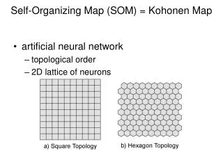
Two distinct properties of SOM • Clustering of multidimensional input data • Spatially ordering the output map so that similar input patterns tend to produce a response in units that are close to each other in the output map. • Topology preserving • nodes in the output layer represent clustering information from the input data (480) 965-6133 (voice) (480) 965-0461 (fax) si@asu.edu
Applications of SOM • Speech processing • Vector quantization • Image coding • Biological signal analysis • Visualize results from multi-dimensional data analysis. • And many many more… (480) 965-6133 (voice) (480) 965-0461 (fax) si@asu.edu
Structure of the presentation • Background • The algorithm • Analysis • Case 1 – motor data analysis • Case 2 – auditory data analysis • Case 3 – supplier change control • A qualitative comparison • Advanced issue – topology preserving • Conclusions (480) 965-6133 (voice) (480) 965-0461 (fax) si@asu.edu
A finite set of nodes Undirected edges adjacent to , if The output map - undirected graph (480) 965-6133 (voice) (480) 965-0461 (fax) si@asu.edu
i c The self-organizing map Output graph G Weight vector W Input vector (480) 965-6133 (voice) (480) 965-0461 (fax) si@asu.edu
Learning the topological mapping from input • The graph (output map) is usually pre-specified as a one-dimensional chain or two dimensional lattice. • SOM intends to learn the topological mapping by means of self-organization driven by samples X • X is assumed to be connected in parallel to every node in the output map. • A node in G, associated with a weight vector W, can be represented by its index i or its position (480) 965-6133 (voice) (480) 965-0461 (fax) si@asu.edu
SOM building block • Find the winner and the neighborhood of the winner • comparing the inner products WiTX, for i = 1,2…L and selecting the node with the largest inner product. • If the weight vectors Wiare normalized, the inner product criterion is equivalent to the minimum Euclidean distance measure. c(X) = arg min ||X-Wi||, i = 1,2…L • With c(X) to indicate the output node of which the weight vector “matches” the input vector X the best (480) 965-6133 (voice) (480) 965-0461 (fax) si@asu.edu
SOM building block (continued) • Adaptive process (by Oja 1982): • The weight vectors inside the neighborhood of the winner are usually updated by Hebbian type learning law. • the negative component is a nonlinear forgetting term. (480) 965-6133 (voice) (480) 965-0461 (fax) si@asu.edu
Discrete-time update format for the adaptive process • Simplifying the equation, • yi(t) = 1 if node i inside the neighborhood of the winner c • yi(t) = 0 otherwise • Obtained discrete-time format (480) 965-6133 (voice) (480) 965-0461 (fax) si@asu.edu
SOM Algorithm implementation 1. Select a winner ‘c’ in the map by : 2. Update the weights in the neighborhood of ‘c’ by Where ‘c’ is the neighborhood function, defined as: (480) 965-6133 (voice) (480) 965-0461 (fax) si@asu.edu
Neighborhood Function • bell-shaped neighborhood Neighborhood is large at first, shrinks over time (480) 965-6133 (voice) (480) 965-0461 (fax) si@asu.edu
square neighborhood (480) 965-6133 (voice) (480) 965-0461 (fax) si@asu.edu
Learning Rate α(t) • Essential for convergence • Large enough for the network to adapt quickly for the new training patterns • Small enough for stability - the network would not forget the experience from the past training patterns • A decreasing function of time. (480) 965-6133 (voice) (480) 965-0461 (fax) si@asu.edu
SOM Software Implementation • Matlab Neural Networks Tool box • SOM toolbox created by a group at the Helsinki Institute of Technology • SOMToolbox downloaded from website at http://www.cis.hut.fi/projects/somtoolbox/about.html (480) 965-6133 (voice) (480) 965-0461 (fax) si@asu.edu
Structure of the presentation • Background • The algorithm • Analysis • Case 1 – motor data analysis • Case 2 – auditory data analysis • Case 3 – supplier change control • A qualitative comparison • Advanced issue – topology preserving • Conclusions (480) 965-6133 (voice) (480) 965-0461 (fax) si@asu.edu
Weight convergence (Assumptions) • the input has discrete probability density • the learning rate α(k) satisfies conditions (Robbins and Monro, 1951): (480) 965-6133 (voice) (480) 965-0461 (fax) si@asu.edu
Weight convergence (Results) • SOM algorithm (locally or globally) minimizes the objective function • Weights converge almost truly to a stationary solution if the stationary solution exists Lin, Si, “Weight Value Convergence of the SOM Algorithm for Discrete Input” (480) 965-6133 (voice) (480) 965-0461 (fax) si@asu.edu
Voronoi polyhedra Voronoi polyhedra on Rn: Masked Voronoi polyhedra on: (480) 965-6133 (voice) (480) 965-0461 (fax) si@asu.edu
Some extreme cases … • Assume neighborhood function is constant Nc(k)=Nc in the final learning phase, then where (480) 965-6133 (voice) (480) 965-0461 (fax) si@asu.edu
Extreme case 1 Neighborhood covers the entire output map, i.e. Each weight vector converges to the same stationary state which is the mass center of the training data set. To eliminate the effect of initial conditions, we should use a neighborhood function covering a large range of the output map. (480) 965-6133 (voice) (480) 965-0461 (fax) si@asu.edu
Extreme case 2 Neighborhood equals 0, i.e. where Wi* become the centroids of the cells of Voronoi partition of the inputs and the final iterations of SOM becomes a sequential updating process of vector quantization. SOM could be used for vector quantization by shrinking the range of the neighborhood function to zero during the learning process. (480) 965-6133 (voice) (480) 965-0461 (fax) si@asu.edu
Observations • Robbins-Monro algorithm ensures weight convergence to the root dJ/dWi=0 almost truly if the root exists. • In practice the weights would only converge to local minima. • It has been observed that SOM is capable to some extent of escaping from local minima when it is used for vector quantization (Mcauliffe 1990). • Topology ordering of weights is not explicitly proved but it remains as a well observed practice in many applications. (480) 965-6133 (voice) (480) 965-0461 (fax) si@asu.edu
Structure of the presentation • Background • The algorithm • Analysis • Case 1 – motor data analysis • Case 2 – auditory data analysis • Case 3 – supplier change control • A qualitative comparison • Advanced issue – topology preserving • Conclusions (480) 965-6133 (voice) (480) 965-0461 (fax) si@asu.edu
Monkey’s motor cortical data analysis to interpret its movement intention Collaborators Andy Schwartz, Siming Lin (480) 965-6133 (voice) (480) 965-0461 (fax) si@asu.edu
Motor Experiment – Overview (480) 965-6133 (voice) (480) 965-0461 (fax) si@asu.edu
I3 I2 I1 time Firing rate calculation dt: bin size, Ti / Tj: start / end time of the i-th bin dij: the firing rate of the i-th bin [Ti , Tj], Tj = Ti+dt. Calculation of dij: the number of spike intervals overlapping with the i-th bin is first determined to be 3. As shown (counting from left to right), 30% of the first interval, 100% of the second interval, and 50% of the third interval are located in the I-th bin. Thus the equation above. (480) 965-6133 (voice) (480) 965-0461 (fax) si@asu.edu
Self-Organizing Application – Motor Cortical Information processing • Spike signal and feature extraction • Computation models using SOM • Visualization of firing patterns of motor cortex • Neural trajectory computation • Weights are adaptively updated by the average discharge rates Input Average discharge rates of 81 cells Output Two-dimensional grid, each node codes the movement directions from the average discharge rates (480) 965-6133 (voice) (480) 965-0461 (fax) si@asu.edu
The Self-Organized Map of Discharge Rates from 81 Neurons in the Center - Out Task (480) 965-6133 (voice) (480) 965-0461 (fax) si@asu.edu
1 8 1 1 7 7 8 7 1 7 7 1 1 8 6 6 2 2 2 6 8 2 6 8 6 2 3 5 5 3 3 4 3 3 4 4 4 5 5 5 The Self-Organized Map of Discharge Rates from 81 Neurons in the Center - Out Task (480) 965-6133 (voice) (480) 965-0461 (fax) si@asu.edu
10 10 10 8 10 7 9 8 7 9 9 11 7 8 11 9 8 8 10 8 7 10 8 7 12 11 12 6 8 7 9 6 6 12 11 13 11 6 6 9 10 12 10 10 5 5 11 13 11 5 5 13 5 4 12 13 12 4 2 13 13 3 14 13 3 4 14 14 2 3 13 14 15 14 2 3 14 15 16 15 3 1 15 15 16 2 1 15 16 1 1 1 15 16 16 15 1 2 1 2 The Self-Organized Map of Discharge Rates – from 81 Neurons in the Spiral Task (480) 965-6133 (voice) (480) 965-0461 (fax) si@asu.edu
Neural Directions: Four Trials for Training, One for Testing in Spiral Task (480) 965-6133 (voice) (480) 965-0461 (fax) si@asu.edu
Neural Trajectory: Four Trials for Training, one for testing Left: monkey finger trajectory; Right: SOM predicted trajectory (480) 965-6133 (voice) (480) 965-0461 (fax) si@asu.edu
Neural Trajectory: Data from Spiral Tasks and Center-out Tasks for Training Left: monkey finger trajectory; Right: SOM predicted trajectory (480) 965-6133 (voice) (480) 965-0461 (fax) si@asu.edu
Neural Trajectory: Average Testing Result from Five Trials Using Leave-K-Out Left: monkey finger trajectory; Right: SOM predicted trajectory (480) 965-6133 (voice) (480) 965-0461 (fax) si@asu.edu
Trajectory Computation Error in 100 Bins (480) 965-6133 (voice) (480) 965-0461 (fax) si@asu.edu
Structure of the presentation • Background • The algorithm • Analysis • Case 1 – motor data analysis • Case 2 – auditory data analysis • Case 3 – supplier change control • A qualitative comparison • Advanced issue – topology preserving • Conclusions (480) 965-6133 (voice) (480) 965-0461 (fax) si@asu.edu
Guinea pig auditory cortical data analysis to interpret its perception of sound Collaborators Russ Witte , Jing Hu, Daryl Kipke (480) 965-6133 (voice) (480) 965-0461 (fax) si@asu.edu
1 mm Surgical implant, neural recordings Sample Signal from a single electrode Microvolts Time (sec) Each of 60 frequencies spanning 6 octaves were repeated 10 times.Each stimulus interval lasted 700ms, including 200ms of tone on time and 500ms of off time(interstimulus interval). (480) 965-6133 (voice) (480) 965-0461 (fax) si@asu.edu
Stream of Neural Activity g180926a Time (sec) Raster Plot- 6s snapshot (480) 965-6133 (voice) (480) 965-0461 (fax) si@asu.edu
Averaged Spike count of 22 chan 1701Hz 1473Hz (480) 965-6133 (voice) (480) 965-0461 (fax) si@asu.edu
Spikerate of Channel1, Stimulus 1-60 (480) 965-6133 (voice) (480) 965-0461 (fax) si@asu.edu
Data Processing • Channel selection - 30 channels were selected • Bin width - Basic unit to hold spike count from experiment data, 5ms, 10ms, 20ms, or higher. 70ms-bin size used • Noise filtering - Apply Gaussian filter to binned data. • Frequency grouping – 12 out of 60 stimuli are selected. It is therefore approximately one frequency per half Octave. • Trial loop selection/leave-1-out - Among the 10 loops of experimental data, take 9 for training, leave one for testing (480) 965-6133 (voice) (480) 965-0461 (fax) si@asu.edu
SOM Training and Testing • Input vector: Bins from all channels are combined. Training/testing patterns are from all loops. • Output: 2-Dimensional grid. The position of each node in the map corresponds to certain spike pattern. • Training parameters: map size (eg 10 10), learning rate (0.02/0.0001), neighborhood function (Gaussian) and radius (eg 10/0), training/fine-tuning epochs, reducing schedules.etc. • Calibration after training: label the output using the labels (frequencies) of the training data (480) 965-6133 (voice) (480) 965-0461 (fax) si@asu.edu
Tonotopic maps: natural vs. SOM 1473 1028 717 Neuronal activities of one channel that leads to the predicted stimulus map - Preserved topology Auditory cortex map Channel 12 has a narrow tuning curve. It is mostly tuned into 700-1500Hz auditory tones. (480) 965-6133 (voice) (480) 965-0461 (fax) si@asu.edu
Results from 10 sessions using leave_k_out (480) 965-6133 (voice) (480) 965-0461 (fax) si@asu.edu