Self Organizing Maps
Self Organizing Maps. Under the Guidance of: Prof. Pushpak Bhattacharya. Mahendra Mani Ojha 01005024 Pranshu Sharma 01005026 Shivendra S. Meena 01005030. Overview. Terminology used Introduction of SOM Components of SOM Structure of the map Training algorithms of the map


Self Organizing Maps
E N D
Presentation Transcript
Self Organizing Maps Under the Guidance of: Prof. Pushpak Bhattacharya Mahendra Mani Ojha 01005024 Pranshu Sharma 01005026 Shivendra S. Meena 01005030
Overview • Terminology used • Introduction of SOM • Components of SOM • Structure of the map • Training algorithms of the map • Advantages and disadvantages • Proof of Convergence • Applications • Conclusion • Reference
Terminology used • Clustering • Unsupervised learning • Euclidean Distance
Introduction of SOM • Introduced by Prof. Teuvo Kohonen in 1982 • Also known as Kohonen feature map • Unsupervised neural network • Clustering tool of high-dimensional and complex data
Introduction of SOM contd… • Maintains the topology of the dataset • Training occurs via competition between the neurons • Impossible to assign network nodes to specific input classes in advance • Can be used for detecting similarity and degrees of similarity • It is assumed that input pattern fall into sufficiently large distinct groupings • Random weight vector initialization
Components of SOM • Sample data • Weights • Output nodes
Structure of the map • 2-dimensional or 1-dimensional grid • Each grid point represents a output node • The grid is initialized with random vectors
Training Algorithm • Initialize Map • For t from 0 to 1 • Select a sample • Get best matching unit • Scale neighbors • Increase t a small amount End for
Initializing the weights • SOMs are computationally very expensive. • Good Initialization • Less iterations • Quality of Map
Get Best Matching Unit • Any method for vector distance i. e. • Nearest neighbor • Farthest neighbor • Distance between means • Distance between medians • Most common method is Euclidean distance. • More than one contestant, choose randomly
Scale Neighbors • Determining Neighbors • Neighborhood size • Decreases over time • Effect on neighbors • Learning
Necessary conditions • Amount of training data • Change of weights should be • In excited neighborhood • Proportional to activation received
Advantages • Very easy to understand • Works well • Disadvantages • computationally expensive • every SOM is different
Proof of convergence • Complete proof only for one dimension. • Very trivial • Almost all partial proofs are based on • Markov chains • Difficulties : • No definition for “A correctly ordered configuration” • Proved result : It is not possible to associate a “Global decreasing potential function” with this algorithm.
WebSOM (overview) • Millions of Documents to be Searched • Keywords or Key phrases used for searching • DATA is clustered • According to similarity • Context • It is kind of a Similarity graph of DATA • For proper storage raw text documents must be encoded for mapping.
Feature Vectors / Encoding • Can simply be histograms of words of the Document. • (Histogram may be the input vector but that makes it a very large Input vector, so there is a need of some kind of reduction) • Reduction • Reduction by random mapping • Weighted word histogram (based on word frequency) • By Latent Semantic Analysis
WebSOM • Architecture • Word category Map • Document category Map • Modes of Operation • Supervised • (some information about the class is given, for e.g. in the collection of Newsgroup articles maybe the name of news group is supplied) • Unsupervised • (no information provided)
Word Category Map • Preprocessing • Remove unimportant data (like images, signatures) • Remove articles prepositions etc. • Words occurring less than some fixed no. of times are to be termed as don’t care ! • Replace synonymous words
Averaging Method • Word code vector • Each word represented by a unique vector (with dimension n ~ 100) • Values may be random • Context Vector • For word at position i word vector is x(i) • where: • E() = Estimate of expected value of x over text corpus • ε = small scalar number
Training: taking words with different x(i)’s Input X(i)’s again . At the best matching node write the corresponding word . Similar context words come at same node (contd.) Example
Document Category Map • Encoded by mapping text word by word onto the WCM. • A histogram is formed based on the hits on WCM. • Use this histogram as fingerprint for DCM.
References [1] T.Honkela, S.Kaski, K.Lagus,T.Kohonen. WEBSOM- Self Organizing Maps of Document Collection. (1997) [2] T.Honkela, S.Kaski, K.Lagus,T.Kohonen. Exploration of full text Databases with Self Organizing Maps. (1996) [3] Teuvo Kohonen. Self-Organization of very large document collections: State of the art (1998) [4] http://websom.hut.fi/websom