Download
1 / 47
480 likes | 613 Views
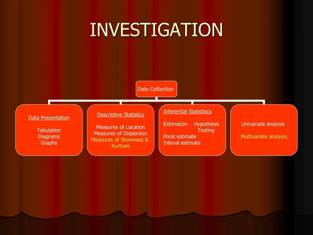
INVESTIGATION. EXAMPLE:. (1) 7,8,9,10,11 n=5, x=45, =45/5=9 (2) 3,4,9,12,15 n=5, x=45, =45/5=9 (3) 1,5,9,13,17 n=5, x=45, =45/5=9 S.D. : (1) 1.58 (2) 4.74 (3) 6.32. Measures of Dispersion Or Measures of variability. Measures of Dispersion.

E N D
EXAMPLE: (1) 7,8,9,10,11 n=5, x=45, =45/5=9 (2) 3,4,9,12,15 n=5, x=45, =45/5=9 (3) 1,5,9,13,17 n=5, x=45, =45/5=9 S.D. : (1) 1.58 (2) 4.74 (3) 6.32
Measures of Dispersion Or Measures of variability
Measures of Dispersion • measures of dispersion summarize differences in the data, how the numbers differ from one another.
Series I: 70 70 70 70 70 70 70 70 70 70 Series II: 66 67 68 69 70 70 71 72 73 74 Series III: 1 19 50 60 70 80 90 100 110 120
A single summary figure that describes the spread of observations within a distribution. Measures of Variability
RANGE INTERQUARTILE RANGE VARIANCE STANDARD DEVIATION MEASURES OF DESPERSION
Range Difference between the smallest and largest observations. Interquartile Range Range of the middle half of scores. Variance Mean of all squared deviations from the mean. Standard Deviation Rough measure of the average amount by which observations deviate from the mean. The square root of the variance. Measures of Variability
Range • The difference between the lowest and highest values in the data set. • The range can be misleading with outliers data: 2,4,5,2,5,6,1,6,8,25,2 Sorted data: 1,2,2,2,3,4,5,6,6,8,25
Hotel Rates 52, 76, 100, 136, 186, 196, 205, 150, 257, 264, 264, 280, 282, 283, 303, 313, 317, 317, 325, 373, 384, 384, 400, 402, 417, 422, 472, 480, 643, 693, 732, 749, 750, 791, 891 Range: 891-52 = 839 Variability Example: Range
Measures of Position Quartiles, Deciles, Percentiles
Quartiles Q1, Q2, Q3 divides ranked scores into four equal parts 25% 25% 25% 25% Q1 Q2 Q3 (minimum) (maximum) (median)
Quartiles: Inter quartile : IQR = Q3 – Q1
The inter quartile range is Q3-Q1 50% of the observations in the distribution are in the inter quartile range. The following figure shows the interaction between the quartiles, the median and the inter quartile range. Inter quartile Range
Sample Number Unsorted Values 1 25 2 27 3 20 4 23 5 26 6 24 7 19 8 16 9 25 10 18 11 30 12 29 13 32 14 26 15 24 16 21 17 28 18 27 19 20 20 16 21 14
Sample Number Unsorted Values Ranked Values 1 25 14 2 27 16 3 20 16 4 23 18 5 26 19 6 24 20 7 19 20 8 16 21 9 25 23 10 18 24 11 30 24 12 29 25 13 32 25 14 26 26 15 24 26 16 21 27 17 28 27 18 27 28 19 20 29 20 16 30 21 14 32
Sample Number Unsorted Values Ranked Values 1 25 14 Minimum 2 27 16 3 20 16 4 23 18 5 26 19 6 24 20 LQ or Q1 7 19 20 8 16 21 9 25 23 10 18 24 11 30 24 Md or Q2 12 29 25 13 32 25 14 26 26 15 24 26 16 21 27 UQ or Q3 17 28 27 18 27 28 19 20 29 20 16 30 21 14 32 Maximum
10% 10% 10% 10% 10% 10% 10% 10% 10% 10% D1 D2 D3 D4 D5 D6 D7 D8 D9 Deciles D1, D2, D3, D4, D5, D6, D7, D8, D9 divides ranked data into ten equal parts
Q1 = P25 Q2 = P50 Q3 = P75 D1 = P10 D2 = P20 D3 = P30 • • • D9 = P90 Deciles Quartiles
Quartiles, Deciles, Percentiles Fractiles (Quantiles) partitions data into approximately equal parts
Maximum is 100th percentile: 100% of values lie at or below the maximum Median is 50th percentile: 50% of values lie at or below the median Any percentile can be calculated. But the most common are 25th (1st Quartile) and 75th (3rd Quartile) Percentiles and Quartiles
A percentile is a score below which a specific percentage of the distribution falls(the median is the 50th percentile. The 75th percentile is a score below which 75% of the cases fall. The median is the 50th percentile: 50% of the cases fall below it Another type of percentile :The quartile lower quartile is 25th percentile and the upper quartile is the 75th percentile Locating Percentiles in a Frequency Distribution
25% included here 25th percentile 50% included here 50th percentile 80thpercentile 80% included here
Five Number Summary • Minimum Value • 1st Quartile • Median • 3rd Quartile • Maximum Value
VARIANCE: Deviations of each observation from the mean, then averaging the sum of squares of these deviations. STANDARD DEVIATION: “ ROOT- MEANS-SQUARE-DEVIATIONS”
The average amount that a score deviates from the typical score. Score – Mean = Difference Score Average of Difference Scores = 0 In order to make this number not 0, square the difference scores (no negatives to cancel out the positives). Variance
Population Sample Variance: Computational Formula
To “undo” the squaring of difference scores, take the square root of the variance. Return to original units rather than squared units. Standard Deviation
Standard deviation: measures the variation of a variable in the sample. Technically, Quantifying Uncertainty
Population Sample Standard Deviation Rough measure of the average amount by which observations deviate on either side of the mean. The square root of the variance.
Example: Data: X = {6, 10, 5, 4, 9, 8}; N = 6 Mean: Variance: Standard Deviation: Total: 42 Total: 28
Marks achieved by 7 students: 3, 4, 6, 2, 8, 8, 5 Mean of these marks = 36/7 = 5.14 Deviations from mean… Example of SD with discrete data Solution! Square them to get rid of the negatives… (x – x)2 Problem! The sum of the deviations is always going to be 0! Total = 0
Example of SD with discrete data • Marks achieved by 7 students: 3, 4, 6, 2, 8, 8, 5 • Mean of these marks = 36/7 = 5.14 • Deviations from mean… (x – x)2 Variance = 32.85 / 7 = 4.69 SD = √4.69 = 2.17 Total = 32.85 Total = 0
Variability Example: Standard Deviation Mean: 6 Standard Deviation: 2
Using the mean and standard deviation together: Is an efficient way to describe a distribution with just two numbers. Allows a direct comparison between distributions that are on different scales. Mean and Standard Deviation
DISTRIBUTION OF DATA IS SYMMETRIC ---- USE MEAN & S.D., DISTRIBUTION OF DATA IS SKEWED ---- USE MEDIAN & QUARTILES WHICH MEASURE TO USE ?
Distributions • Bell-Shaped (also known as symmetric” or “normal”) • Skewed: • positively (skewed to the right) – it tails off toward larger values • negatively (skewed to the left) – it tails off toward smaller values