Download
1 / 68
680 likes | 691 Views
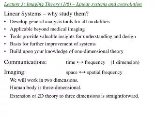
Lecture: Linear systems and convolution. Linearity Conditions. Let f 1 (x,y) and f 2 (x,y) describe two objects we want to image. f 1 (x,y) can be any object and represent any characteristic of the object. (e.g. color, intensity, temperature, texture, X-ray absorption, etc.)

E N D
Linearity Conditions Let f1(x,y) and f2(x,y) describe two objects we want to image. f1(x,y) can be any object and represent any characteristic of the object. (e.g. color, intensity, temperature, texture, X-ray absorption, etc.) Assume each is imaged by some imaging device (system). Let f1(x,y) → g1(x,y) f2(x,y) → g2(x,y) Let’s scale each object and combine them to form a new object. a f1(x,y) + b f2(x,y) If the system is linear, output is a g1(x,y) + b g2(x,y)
Linearity Example: Is this a linear system?
Linearity Example: Is this a linear system? 9 → 3 16→ 4 9 + 16 = 25 → 5 3 + 4 ≠ 5 Not linear.
Example in medical imaging: Doubling the X-ray photons → doubles those transmitted Doubling the nuclear medicine → doubles the reception source energy MR: Maximum output voltage is 4 V. Now double the water: The A/D converter system is non-linear after 4 mV. (overranging)
Linearity allows decomposition of functions Linearity allows us to decompose our input into smaller, elementary objects. Output is the sum of the system’s response to these basic objects.
Elementary Function: The two-dimensional delta function δ(x,y) δ(x,y) has infinitesimal width and infinite amplitude. Key: Volume under function is 1. δ(x,y)
The delta function as a limit of another function Powerful to express δ(x,y) as the limit of a function Gaussian: lim a2 exp[- a2(x2+y2)] =δ(x,y) 2D Rect Function: lim a2 Π(ax)Π(ay) = δ(x,y) where Π(x) = 1 for |x| < ½ For this reason, δ(bx) = (1/|b|) δ(x)
Sifting property of the delta function The delta function at x1 = ε, y1= η has sifted out f (x1,y1) at that point. One can view f (x1,y1) as a collection of delta functions, each weighted by f (ε,η).
Imaging Analyzed with System Operators Let system operator (imaging modality) be , so that From previous page: Why the new coordinate system (x2,y2)?
Imaging Analyzed with System Operators Then, Generally System operating on entire blurred object input object f1 (x1,y1) By linearity, we can consider the output as a sum of the outputs from all the weighted elementary delta functions. Then,
System response to a two-dimensional delta function Substituting this into yields the Superposition Integral
Example in medical imaging: Consider a nuclear study of a liver with a tumor point source at x1 = ε, y1= η Radiation is detected at the detector plane. To obtain a general result, we need to know all combinations h(x2, y2; ε, η) By “general result”, we mean that we could calculate the image I(x2, y2) for any source input S(x1, y1)
Time invariance A system is time invariant if its output depends only on relative time of the input, not absolute time. To test if this quality exists for a system, delay the input by t0. If the output shifts by the same amount, the system is time invariant i.e. f(t)→ g(t) f(t - to) → g(t - to) input delay output delay Is f(t)→ f(at) → g(t) (an audio compressor) time invariant?
Time invariance A system is time invariant if its output depends only on relative time of the input, not absolute time. To test if this quality exists for a system, delay the input by t0. If the output shifts by the same amount, the system is time invariant i.e. f(t)→ g(t) f(t - to) → g(t - to) input delay output delay Is f(t)→ f(at) → g(t) (an audio compressor) time invariant? f(t - to) → f(at) → f(a(t – to)) - output of audio compressor f(at – to) - shifted version of output (this would be a time invariant system.) So f(t)→ f(at) = g(t) is not time invariant.
Space or shift invariance A system is space (or shift) invariant if its output depends only on relative position of the input, not absolute position. If you shift input → The response shifts, but in the plane, the shape of the response stays the same. If the system is shift invariant, h(x2, y2; ε, η) = h(x2-ε , y2-η) and the superposition integral becomes the 2D convolution function: Notation: g = f**h (** sometimes implies two-dimensional convolution, as opposed to g = f*h for one dimension. Often we will use * with 2D and 3D functions and imply 2D or 3D convolution.)
One-dimensional convolution example: g(x) = Π(x)*Π(x/2) Recall: Π(x) = 1 for |x| < ½ Π(x/2) = 1 for |x|/2 < ½ or |x| < 1 Flip one object and drag across the other. flip delay
One-dimensional convolution example, continued: Case 1: no overlap of Π(x-x’) and Π(x’/2) Case 2: partial overlap of Π(x-x’) and Π(x’/2)
One-dimensional convolution example, continued(2): Case 3: complete overlap Case 4: partial overlap Case 5: no overlap
One-dimensional convolution example, continued(3): Result of convolution:
Two-dimensional convolution sliding of flipped object
تبدیل فوریه (Fourier Transform) • پس ازعبور نور از يك منشور (Prism) يا diffraction grating، نور به اجزا مختلف با فركانس هاي خاص خود (مونوكروماتيك) تجزيه مي شود. • اين امر مشابه تبديل فوريه (FT) است. • مي توان يــك سيگنال يك بعدي را بصورت مجموعه اي از امواج سينوسي (با فركانس و دامنه متفاوت) نشان داد. • هرچه فركانس هاي بيشتري را محاسبه نماييم تخمين فوريه يك سيگنال دقيق تر مي شود و اطلاعات بيشتري درباره شكل اوليه آن بدست مي آيد.
تبدیل فوریه (Fourier Transform) • FT مبتني بر اين واقعيت است كه سيگنال دوره اي (Periodic) شامل بي نهايت سيگنال هاي سينوسي وزن دار با فــركانس هاي متفاوت است. اين فركانس ها عبارتند از فركانس پايه (frequencyFundamental ) و مضارب درست اين فركانس پايه. • در تبديل فوريه، توابع پايهاي هم جهت(orthonormal basis function)، امواج سينوسي با فركانسهاي متفاوت هسنند كه در فضاي بينهايت تعريف شدهاند
تبدیل فوریه (Fourier Transform) • هر يك از ضرايب حاصل در تبديل فوريه توسط ضرب نقطهاي(inner product) تابع ورودي و يكي از توابع پايهاي(basis function) بدست ميآيد. • اين ضرايب، در واقع، درجه شباهت بين تابع ورودي و تابع پايهاي مورد نظر را نشان ميدهد. • اگر دو تابع پايهاي بر هم عمود(orthogonal) باشند، حاصلضرب نقطهاي آنها صفر و لذا نشان ميدهد كه آندو با هم شبيه نيستند. • بنابراين اگر سيگنال يا تصوير ورودي از اجزايي تشكيل شده باشد كه يك يا چند تابع پايهاي داشته باشد، سپس آن يك يا چند ضريب بزرگ و ديگر ضرايب كوچك هستند.
Inverse Fouriers Transform • در تبديل معكوس، سيگنال يا تصوير اوليه توسط مجموع توابع پايهاي (در فركانسهاي مختلف) كه تحت تاثير وزن ضرايب تبديل قرار گرفتهاند، بازسازي ميشود. • بنابراين اگر يك سيگنال يا تصوير از اجزائي شبيه به تعداد معدودي از توابع پايهاي تشكيل شده باشد، بسياري از عبارات موجود در اين جمع (ضرايب تبديل) حذف شده و فقط تعدادي از اين ضرايب تبديل، تقويت اجزايي از تصوير را كه شبيه به توابع مربوطه پايهاي است انجام داده و تصوير را ميسازند.
Advantage • وقتي تبديل فوريه يك سيگنال يا تصوير بدست مي آيد، اعمال متعدد رياضي برروي آنها قابل انجام است. در فضاي فركانسي انجام اين عمليات رياضي از انجام آنها در فضاي مكاني به مراتب ساده تر است. • بعنوان مثال عمل Convolution به يك ضرب ساده تبديل مــي شود و روش هاي پردازشي ديگر نيز مانند Correlation، differentiation، integration و Interpolation به سهولت انجام مي شوند.
Fourier Transform: Inverse Fourier Transform: 1-D Fourier Theory You may have seen the Fourier transform and its inverse written as: • Why use the top version instead? • No scaling factor (1/2); easier to remember. • Easier to think in Hz than in radians/s
Review of 1-D Fourier Theory, continued Fourier Transform: Let’s generalize so we can consider functions of variables other than time. Inverse Fourier Transform:
Review of 1-D Fourier theory, continued (2) F(u) gives us the magnitude and phase of each of the exponentials that comprise f(x). In fact, the Fourier integral works by sifting out the portion of f(x) that is comprised of the the function exp(+i 2π uox). Orthogonal basis functions f(x) can be viewed as as a linear combination of the complex exponential basis functions.
Some Fourier Transform Pairs and Definitions -1/2 1/2 -1 1
MX (Real) MY (Imaginary)
MX (Real) MY (Imaginary)
1-D Fourier transform properties If f(x) ↔ F(u) and h(x) ↔ H(u) , Linearity: af(x) + bh(x) ↔ aF(u) + bH(u) Scaling: f(ax) ↔ Shift: f(x-a) ↔
1-D Fourier transform properties, continued. Say g(x) ↔ G(u). Then, Derivative Theorem: (Emphasizes higher frequencies – high pass filter) Integral Theorem: (Emphasizes lower frequencies – low pass filter)
Even and odd functions and Fourier transforms Any function g(x) can be uniquely decomposed into an even and odd function. e(x) = ½( g(x) + g(-x) ) o(x) = ½( g(x) – g(-x) ) For example, e1 · e2 = even o1 · o2 = even e1 · o1 = odd e1 + e2 = even o1 + o2 = odd
Fourier transforms of even and odd functions Consider the Fourier transforms of even and odd functions. g(x) = e(x) + o(x) Sidebar: E(u) and O(u) can both be complex if e(x) and o(x) are complex. If g(x) is even, then G(u) is even. If g(x) is odd, then G(u) is odd.
Special Cases For a real-valued g(x) ( e(x) , o(x) are both real ), Real part is even in u Imaginary part is odd in u So, G(u) = G*(-u), which is the definition of Hermitian Symmetry: G(u) = G*(-u) (even in magnitude, odd in phase)
Example problem Find the Fourier transform of