Download
1 / 12
120 likes | 133 Views
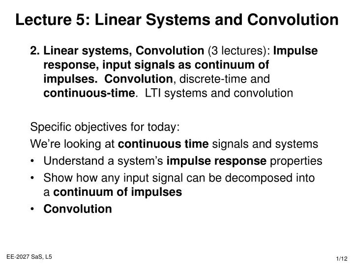
Lecture 5: Linear Systems and Convolution. 2. Linear systems, Convolution (3 lectures): Impulse response, input signals as continuum of impulses. Convolution , discrete-time and continuous-time . LTI systems and convolution Specific objectives for today:

E N D
Lecture 5: Linear Systems and Convolution • 2. Linear systems, Convolution (3 lectures): Impulse response, input signals as continuum of impulses. Convolution, discrete-time and continuous-time. LTI systems and convolution • Specific objectives for today: • We’re looking at continuous time signals and systems • Understand a system’s impulse response properties • Show how any input signal can be decomposed into a continuum of impulses • Convolution
Lecture 5: Resources • Core material • SaS, O&W, C2.2 • Background material • MIT lecture 4
Introduction to “Continuous” Convolution • In this lecture, we’re going to understand how the convolution theory can be applied to continuous systems. This is probably most easily introduced by considering the relationship between discrete and continuous systems. • The convolution sum for discrete systems was based on the sifting principle, the input signal can be represented as a superposition (linear combination) of scaled and shifted impulse functions. • This can be generalised to continuous signals, by thinking of it as the limiting case of arbitrarily thin pulses
Signal “Staircase” Approximation • As previously shown, any continuous signal can be approximated by a linear combination of thin, delayed pulses: • Note that this pulse (rectangle) has a unit integral. Then we have: • Only one pulse is non-zero for any value of t. Then as D0 • When D0, the summation approaches an integral • This is known as the sifting property of the continuous-time impulse and there are an infinite number of such impulses d(t-t) dD(t) 1/D D
Alternative Derivation of Sifting Property • The unit impulse function, d(t), could have been used to directly derive the sifting function. • Therefore: • The previous derivation strongly emphasises the close relationship between the structure for both discrete and continuous-time signals
Continuous Time Convolution • Given that the input signal can be approximated by a sum of scaled, shifted version of the pulse signal, dD(t-kD) • The linear system’s output signal y is the superposition of the responses, hkD(t), which is the system response to dD(t-kD). • From the discrete-time convolution: • What remains is to consider as D0. In this case: ^ ^
Example: Discrete to Continuous Time Linear Convolution • The CT input signal (red) x(t) is approximated (blue) by: • Each pulse signal • generates a response • Therefore the DT convolution response is • Which approximates the CT convolution response
Linear Time Invariant Convolution • For a linear, time invariant system, all the impulse responses are simply time shifted versions: • Therefore, convolution for an LTI system is defined by: • This is known as the convolution integral or the superposition integral • Algebraically, it can be written as: • To evaluate the integral for a specific value of t, obtain the signal h(t-t) and multiply it with x(t) and the value y(t) is obtained by integrating over t from – to . • Demonstrated in the following examples
Example 1: CT Convolution • Let x(t) be the input to a LTI system with unit impulse response h(t): • For t>0: • We can compute y(t) for t>0: • So for all t: In this example a=1
Example 2: CT Convolution • Calculate the convolution of the following signals • The convolution integral becomes: • For t-30, the product x(t)h(t-t) is non-zero for -<t<0, so the convolution integral becomes:
Lecture 5: Summary • A continuous signal x(t) can be represented via the sifting property: • Any continuous LTI system can be completely determined by measuring its unit impulse response h(t) • Given the input signal and the LTI system unit impulse response, the system’s output can be determined via convolution via • Note that this is an alternative way of calculating the solution y(t) compared to an ODE. h(t) contains the derivative information about the LHS of the ODE and the input signal represents the RHS.
Lecture 5: Exercises • SaS, O&W Q2.8-2.14 • Use the DT conv() function in Matlab (see lecture 4) to sample x() and h() in examples 1 & 2 and check that the analytic results correspond to the approximate discrete values.