Download
1 / 42
420 likes | 653 Views
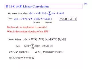
11-C 計算 Linear Convolution. We know that when. then. ( N -point). ( M -point). But how do we implement it correctly? . What is the number of points of the FFT ? . Note: When . then. FFT P : P -point FFT. IFFT L : P -point inverse FFT. (( a )) P : a 除以 P 的餘數.

E N D
11-C 計算 Linear Convolution We know that when then (N-point) (M-point) But how do we implement it correctly? What is the number of points of the FFT? Note: When then FFTP: P-point FFT IFFTL: P-point inverse FFT ((a))P: a除以 P的餘數
Convolution 有幾種 Cases Case 1: Both x[n] and h[n] have infinite lengths. Case 2: Both x[n] and h[n] have finite lengths. Case 3:x[n] has infinite length but h[n] has finite length. Case 4:x[n] has finite length but h[n] has infinite length.
Case 2: Both x[n] and h[n] have finite lengths. x[n] 的範圍為 n [n1, n2],大小為 N = n2− n1 + 1 h[n] 的範圍為 n [k1, k2],大小為 K = k2 − k1 + 1 y[n] 的範圍? y[n] h[n] x[n] n n n n1 n2 k1 k2 n1+k1 n2+k2 N K N+K-1 Convolution output 的範圍以及 點數,是學信號處理的人必需了解的常識
x[n] 的範圍為 n [n1, n2],範圍大小為 N = n2− n1 + 1 h[n] 的範圍為 n [k1, k2],範圍大小為 K = k2 − k1 + 1 當 n固定時 什麼情況下y[n] 有值? 其中至少有一個落在 [n1, n2 ] 的範圍內
n− k2 n− k1 n− k的範圍 n1 n2 x[n] 有值的範圍 必需有交集 n 的下限為 n− k1 與 n1相重合 n − k1 = n1, n = k1 + n1 n 的上限為 n − k2 與 n2相重合 n − k2 = n2, n = k2 + n2 所以 y[n] 的範圍是 n [k1 + n1 , k2 + n2] 範圍大小為 k2 + n2 − k1 − n1 + 1 = N + K − 1
FFT implementation for Case 2 for n = 0, 1, 2, … , N−1 for n = N, N+1 , … , P−1 PN + K − 1 for n = 0, 1, 2, … , K−1 for n = K, K+1 , … , P−1 for n = n1+k1 , n1+k1+1, n1+k1+2, ……., k2 + n2 i.e., 取 output 的前面 N+K1 個點
證明: (from page 355) (h1[k'] = 0 for k K) 可以簡化為 這是因為只有當 時 由於 當 時, 因為 PN + K − 1 , P −K+ 1 N 又 x1[n] = 0 for n N and n < 0 所以當 時
Case 3:x[n] has finite length but h[n] has infinite length x[n] 的範圍為 n [n1, n2],範圍大小為 N = n2− n1 + 1 h[n] 無限長 y[n] 每一點都有值 (範圍無限大) 但我們只想求出 y[n] 的其中一段 希望算出的 y[n] 的範圍為 n [m1, m2],範圍大小為 M = m2 − m1 + 1 h[n] 的範圍 ? 要用多少點的 FFT ?
改寫成 當n = m1 當n = m2
m1− n2 m1− n1 (n = m1) m1−n2+1 m1−n1+1 (n = m1+1) m1−n2+2 m1−n1+2 (n = m1+2) n = m1時n− s的範圍 n = m1 +1 時n− s的範圍 m2−n2 (n = m2) n = m1 +2 時n− s的範圍 n = m2時n− s的範圍 此圖為n− s範圍示意圖 m2−n1 有用到的 h[k] 的範圍:k [m1− n2, m2− n1]
所以有用到的 h[k] 的範圍是 k [m1 −n2 , m2 −n1 ] 範圍大小為 m2 − n1 − m1 + n2 + 1 = N + M − 1 FFT implementation for Case 3 for n = 0, 1, 2, … , N−1 for n = N, N + 1, N + 2, ……, P −1 PN + M − 1 for n = 0, 1, 2, … , L−1 for n = m1, m1+1, m1+2, … , m2 注意:y[n] 只選 y1[n] 的第 N個點到第 N+M1 個點
Suppose that x[n]: input, h[n]: the impulse response of the filter length(x[n]) = N, length(h[n]) = M (Both of them have finite lengths) We want to compute , y[n] = x[n] h[n]. The above convolution needs the P-point DFT, PM + N 1. complexity: O(P log2P) 11-DRelations between the Signal Length and the Convolution Algorithm
Case 1:When M is a very small integer: Directly computing Number of multiplications for directly computing: NM When 3NM 9/2(N + M 1)log2(N + M 1), i.e.,M (3/2)log2N, (粗略估計) it is proper to do directly computing instead of applying the DFT.
Example: N = 126, M = 3, (difference, edge detection) (3/2)log2N = 10.4659 When compute the number of real multiplications explicitly, using direct implementation: 3NM = 1134, using the 128-point DFT: using the 144-point DFT:
Although in usual “directly computing” is not a good idea for convolution implementation, in the cases where (a) M is small (b) The filter has some symmetric relation using the directly computing method may be efficient for convolution implementation. Example: edge detection, smooth filter
Case 2: When M is not a very small integer but much less than N (N >> M): It is proper to divide the input x[n] into several parts: Each part has the size of L (L > M). x[n] (n = 0, 1, …., N1) x1[n], x2[n], x3[n], …….., xS[n] S = N/L, means rounding toward infinite Section 1 x1[n] = x[n] for n = 0, 1, 2, …., L1, Section 2x2[n] = x[n + L] for n = 0, 1, 2, …., L1, : Section sxs[n] = x[n + (s-1)L] for n = 0, 1, 2, …., L1, s = 1, 2, 3, …., S
length = L length = M It should perform the P-point FFTs 2S+1 times or 2S times Why? P L+M1
number of multiplications for the P-point DFT 運算量:2S [(3P/2)log2P] + 3SPSN/L, P L+M1 (linear with N) 何時為optimal?
L (section length) M (filter length)
注意: (1) Optimal section length is independent to N (2) If M is a fixed constant, then the complexity is linear with N, i.e., O(N) 比較:使用原本方法時, complexity = O((N+M-1)log2 (N+M-1)) (3) 實際上,需要考量 P-point FFT 的乘法量必需不多 P= L+M1 例如,根據 page 373 的方法,算出當 M = 10 時, L = 41.5439 為 optimal 但實際上,應該選 L = 39,因為此時 P = L+M1 = 48 點的 DFT 有較少的乘法量
Case 3 When M has the same order as N Case 4 When M is much larger than N Case 5 When N is a very small integer
Sectioned Convolution for the Condition where One Sequence is Finite and the Other One is Infinite x[n] 0 for n1nn2, length of x[n] = N = n2n1 + 1, length of h[n] is infinite, and we want to calculate y[m] for m1mm2, M = m2m1 + 1. Suppose that M << N. In this case, we can try to partition x[n] into several sections. section 1: x1[n] = x[n] for n = n1 ~ n1 + L 1, x1[n] = 0 otherwise, section 2: x2[n] = x[n] for n = n1+ L ~ n1 + 2L 1, x2[n] = 0 otherwise, section q: xq[n] = x[n] for n = n1+ (q1)L ~ n1 + qL 1, xq[n] = 0 otherwise,
Then we perform the convolution of xq[n] * h[n] for each of the sections by the method on pages 365 and 366. (Since the length of xq[n] is L, it requires the P-point DFT, P L+M1. Its complexity and the optimal section length can also be determined by the formulas on page 373.
12. Fast Algorithm 的補充 12-A Discrete Fourier Transform for Real Inputs DFT: 當 f [n] 為 real 時, F [m] = F*[N− m] *: conjugation
若我們要對兩個 real sequences f1[n] ,f2[n] 做 DFTs Step 1: f3[n] = f1[n] + j f2[n] Step 2: F3[m] = DFT{f3[n]} Step 3: 只需一個 DFT 證明:由於 DFT 是一個 linear operation 又 F1[m] = F1*[N − m] F2[m] = F2*[N − m]
同理,當兩個 inputs 為 (1) pure imaginary (2) one is real and another one is pure imaginary 時,也可以用同樣的方法將運算量減半
若 input sequence 為 even f[n] = f[N-n], • 則 DFT output 也為 even F[n] = F[N-n] • 若 input sequence 為 odd f[n] = -f[N-n], • 則 DFT output 也為 odd F[n] = -F[N-n] 若 input sequence 為 odd and real, 則乘法量可減為 1/4
一般的linear operation: (習慣上,把 k[m, n] 稱作 “kernel”) n = 0, 1, …., N1, m = 0, 1, …., M1 可以用矩陣(matrix) 來表示 運算量為 MN 若為linear time-invariant operation: k[m, n] = h[mn] (dependent on m, n之間的差) n = 0, 1, …., N1, m = 0, 1, …., M1 mn的範圍: 從 1N到 M1, 全長M + N 1 運算量為 Llog2L,LM+2N 2 383 12-B Converting into Convolution
大致上,變成 convolution 後 總是可以節省運算量 例子A 可以改寫為 (注意,最後一項為 convolution) 運算量為2N + Llog2L 例子B Linear Canonical Transform 384
通則: 當k[m, n] 可以拆解成 A[m] B[m−n] C[n] 或 即可以使用 convolution
12-C Recursive Method for Convolution Implementation u[n]: unit step function Only two multiplications required for calculating each output.
12-D LUT LUT (lookup table) 道理和背九九乘法表一樣 記憶體容量夠大時可用的方法 Problem: memory requirement wasting energy
附錄十二 創意思考 New ideas 聽起來偉大,但大多是由既有的 ideas 變化而產生 (1) Combination (2) Analog (3) Connection (4) Generalization (5) Simplification (6) Reverse 註:感謝已過逝的李茂輝教授,他開的課「創造發明工程」, 讓我一生受用無窮
(7) Key Factor (8) Imagination (9) 純粹意外
(1) Combination 例: A (existing) B (existing) 蒸汽機 車 火車 C (innovation) (2) Analog 例: continuous Fourier transform continuous cosine transform A (existing) C (existing) B (existing) D (innovation) discrete Fourier transform discrete cosine transform
(3) Connection A (existing) C (innovation) B (existing) 例: 古典物理學 未能解釋的光學現象 相對論 (4) Generalization 例: A (existing) Walsh transform 保留某些特性 將其他特性推廣化 保留不需乘法 將 1 推廣為2k B (innovation) Jacket transform
(5) Simplification 例: DFT A (existing) 保留 orthogonal, 正負號變化 去除 無理數乘法 保留某些特性 去除複雜化的因素 B (innovation) Walsh transform (6) Reverse A (existing) D (innovation) 電 磁生電 (法拉第定律) B (existing) C (existing) 電生磁 磁 (安培定律)
個人做研究時,關於發明創造的心得 (1) 研究問題的第一步,往往是先想辦法把問題簡化 如果不將複雜的經濟問題簡化成二維供需圖,經濟學也就無從發展起來 如果不將電子學的問題簡化常小訊號模型,電子電路的許多問題都將難以解決 個人在研究影像處理時,也常常先針對 size 很小,且較不複雜的影像來做處理,成功之後再處理 size 較大且較複雜的影像 問題簡化之後,才比較容易對問題做分析,並提出改良之道 (2) 如果有好點子,趕快用筆記下來, 好點子是很容易稍縱即逝而忘記的。 (3) 練習多畫系統圖 系統圖畫得越多,越容易發現新的點子
(4) 目前流行一種說法,認為創意來自右腦,而掌管邏輯分析的左腦無助於創造,其實這未必是正確的。 很多時候,對一個問題分析得越清楚,越有系統,反而越能掌握問題的關鍵,而有助於創造 (5) 其實,對台大的同學而言,提出 newideas 並不難,但是要把 ideas 變成有用的、成功的 ideas,不可以缺少分析和解決問題的能力 很少有一個 new idea 一開始就 works well for any case,任何一個成功的創意,都是經由問題的分析,解決一連串的技術上的問題,才產生出來的 (6) 當心情放鬆時,想像力特別強,有助於發現意外的點子。 (7) 就短期而言,技術性的問題固然重要 但是就長期而言,不要因為技術上的困難,而否定了一個偉大的構想
大學以前的教育,是學習前人的智慧結晶 研究所的教育,是訓練創造發明和解決問題的能力
問題思考 如果要濾掉高頻的雜訊,先做 DFT,再將高頻的部分都變成 0 再做 inverse DFT 不就行了? for m ≦ m0 and m ≧ N – m0 for m0 < m < N – m0 那麼…..為什麼要用有點複雜的 FIR filter?