Download
1 / 18
200 likes | 527 Views
Lecture 6: Linear Systems and Convolution. 2. Linear systems, Convolution (3 lectures): Impulse response, input signals as continuum of impulses. Convolution, discrete-time and continuous-time. LTI systems and convolution Specific objectives for today: Properties of an LTI system

E N D
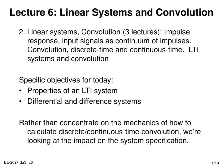
Lecture 6: Linear Systems and Convolution • 2. Linear systems, Convolution (3 lectures): Impulse response, input signals as continuum of impulses. Convolution, discrete-time and continuous-time. LTI systems and convolution • Specific objectives for today: • Properties of an LTI system • Differential and difference systems • Rather than concentrate on the mechanics of how to calculate discrete/continuous-time convolution, we’re looking at the impact on the system specification.
Lecture 6: Resources • Core material • SaS, Oppenheim & Willsky, C2.3-4 • Background material • MIT Lectures 3 & 4 • Health Warning • The following applies to LTI systems only. • For most of the properties, it is possible to find a simple non-linear system which is a counter example to the given properties
LTI Systems and Impulse Response • Any continuous/discrete-time LTI system is completely described by its impulse response through the convolution: • This only holds for LTI systems as follows: • Example: The discrete-time impulse response • Is completely described by the following LTI • However, the following systems also have the same impulse response • Therefore, if the system is non-linear, it is not completely characterised by the impulse response
Commutative Property • Convolution is a commutative operator (in both discrete and continuous time), i.e.: • For example, in discrete-time: • and similar for continuous time. • Therefore, when calculating the response of a system to an input signal x[n], we can imagine the signal being convolved with the unit impulse response h[n], or vice versa, whichever appears the most straightforward.
h1(t) h2(t) Distributive Property (Parallel Systems) • Another property of convolution is the distributive property • This can be easily verified • Therefore, the two systems: • are equivalent. The convolved sum of two impulse responses is equivalent to considering the two equivalent parallel system (equivalent for discrete-time systems) y1(t) x(t) y(t) x(t) y(t) h1(t)+h2(t) + y2(t)
Example: Distributive Property • Let y[n] denote the convolution of the following two sequences: • x[n] is non-zero for all n. We will use the distributive property to express y[n] as the sum of two simpler convolution problems. Let x1[n] = 0.5nu[n], x2[n] = 2nu[-n], it follows that • and y[n] = y1[n]+y2[n], where y1[n] = x1[n]*h[n], y1[n] = x1[n]*h[n]. • From Lecture 3 - example 3, and O&W example 2.5
x(t) w(t) y(t) h1(t) h2(t) Associative Property (Serial Systems) Another property of (LTI) convolution is that it is associative Again this can be easily verified by manipulating the summation/integral indices Therefore, the following four systems are all equivalent and y[n] = x[n]*h1[n]*h2[n] is unambiguously defined. This is not true for non-linear systems (y1[n] = 2x[n], y2[n] = x2[n]) x(t) y(t) h1(t)*h2(t) x(t) y(t) x(t) v(t) y(t) h2(t)*h1(t) h2(t) h1(t)
LTI System Memory • An LTI system is memoryless if its output depends only on the input value at the same time, i.e. • For an impulse response, this can only be true if • Such systems are extremely simple and the output of dynamic engineering, physical systems depend on: • Preceding values of x[n-1], x[n-2], … • Past values of y[n-1], y[n-2], … • for discrete-time systems, or derivative terms for continuous-time systems
x(t) w(t) y(t) h(t) h1(t) System Invertibility • Does there exist a system with impulse response h1(t) such that y(t)=x(t)? • Widely used concept for: • control of physical systems, where the aim is to calculate a control signal such that the system behaves as specified • filtering out noise from communication systems, where the aim is to recover the original signal x(t) • The aim is to calculate “inverse systems” such that • The resulting serial system is therefore memoryless
Example: Accumulator System • Consider a DT LTI system with an impulse response • h[n] = u[n] • Using convolution, the response to an arbitrary input x[n]: • As u[n-k] = 0 for n-k<0 and 1 for n-k0, this becomes • i.e. it acts as a running sum or accumulator. Therefore an inverse system can be expressed as: • A first difference (differential) operator, which has an impulse response
Causality for LTI Systems • Remember, a causal system only depends on present and past values of the input signal. We do not use knowledge about future information. • For a discrete LTI system, convolution tells us that • h[n] = 0 for n<0 • as y[n] must not depend on x[k] for k>n, as the impulse response must be zero before the pulse! • Both the integrator and its inverse in the previous example are causal • This is strongly related to inverse systems as we generally require our inverse system to be causal. If it is not causal, it is difficult to manufacture!
LTI System Stability • Remember: A system is stable if every bounded input produces a bounded output • Therefore, consider a bounded input signal • |x[n]| < B for all n • Applying convolution and taking the absolute value: • Using the triangle inequality (magnitude of a sum of a set of numbers is no larger than the sum of the magnitude of the numbers): • Therefore a DT LTI system is stable if and only if its impulse response is absolutely summable, ie Continuous-time system
Example: System Stability • Are the DT and CT pure time shift systems stable? • Are the discrete and continuous-time integrator systems stable? Therefore, both the CT and DT systems are stable: all finite input signals produce a finite output signal Therefore, both the CT and DT systems are unstable: at least one finite input causes an infinite output signal
Differential and Difference Equations • Two extremely important classes of causal LTI systems: • 1) CT systems whose input-output response is described by linear, constant-coefficient, ordinary differential equations with a forced response • 2) DT systems whose input-output response is described by linear, constant-coefficient, difference equations • Note that to “solve” these equations for y(t) or y[n], we need to know the initial conditions • Examine such systems and relate them to the system properties just described RC circuit with: y(t) = vc(t), x(t) = vs(t), a = b = 1/RC. Simple bank account with: a = -1.01, b = 1.
Continuous-Time Differential Equations • A general Nth-order LTI differential equation is • If the equation involves derivative operators on y(t) (N>0) or x(t), it has memory. • The system stability depends on the coefficients ak. For example, a 1st order LTI differential equation with a0=1: • If a1>0, the system is unstable as its impulse response represents a growing exponential function of time • If a1<0 the system is stable as its impulse response corresponds to a decaying exponential function of time
Discrete-Time Difference Equations • A general Nth-order LTI difference equation is • If the equation involves difference operators on y[n] (N>0) or x[n], it has memory. • The system stability depends on the coefficients ak. For example, a 1st order LTI difference equation with a0=1: • If a1>1, the system is unstable as its impulse response represents a growing power function of time • If a1 <1 the system is stable as its impulse response corresponds to a decaying power function of time
Lecture 6: Summary • The standard notions of commutative, associative and distributive properties are valid for convolution operators. These can be used to simplify evaluating convolution, by decomposing the input system/signal into simpler parts, and then solving the transformed problem. • Standard system notations of • Memory • Causality • Invertibility • Stability • Can be given specific definitions in terms of representing a system via its convolution response or in terms of the derivative/differential equation
Lecture 6: Exercises • Verify the convolution calculation discussed on Slide 6 • SaS, O&W Q2.14-19 • Make sure you have attempted the Matlab/Simulink exercises up to week 5.