Download

1 / 38
380 likes | 456 Views
Explore the effects of terrain on PBL structure, flow over hills, heterogeneous surfaces, and surface roughness variations. Learn through observations and models, addressing current understanding and outstanding issues.

E N D
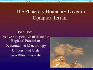
Observations and Models of Boundary-Layer Processes Over Complex Terrain • What is the planetary boundary layer (PBL)? • What are the effects of irregular terrain on the basic PBL structure? • How do we observe the PBL over complex terrain? • What do models tell us? • What is our current understanding of the PBL and what are the outstanding problems to be addressed?
Effects of irregular terrain on PBL structure • Flow over hills (horizontal scale a few km; vertical scale a few 10’s of m up to a fraction of PBL depth) • Flow over heterogeneous surfaces (small-scale variability with discontinuous changes in surface properties)
Flow over a hill (neutral stability) • Idealized profile (Witch of Agnesi profile): (After Maria Agnesi; Milano, Italy, 1748)
Regions of Flow Over Hills • Inner layer – region where turbulent stresses affect changes in mean flow. Hunt et al. (1988) obtain the relation for ℓ: • Outer layer – height at which shear in upwind profile ceases to be important: • For h = 10 m, Lh = 200 m and z0 = 0.02 m, ℓ = 10 m and hm = 66 m
Effects of horizontal heterogeneity in surface properties • Changes in surface roughness • Rough to smooth • Smooth to rough • Changes in surface energy fluxes • Sensible heat flux • Latent heat flux • Changes in incoming solar radiation • Cloudiness • Slope
Scale of changes in PBL downwind of discontinuity • Confined to surface layer (10 to 50 m) • Entire PBL (10 to 100 km) • Mesoscale (geostrophic adjustment; > 100 km)
Changes in surface roughness • Characterized by change in roughness length – • , where upwind roughness length and downwind roughness length
Surface-layer internal boundary layer We define internal BL by (subscript θ for temperature and c for other scalars). The simplest formulations for are of the form (analogous to BL growth on a smooth flat plate in wind tunnel experiments.) ,
Surface-layer internal boundary layer A more sophisticated approach is to assume vertical diffusion then, With at With this gives reasonable agreement With observations. (Works best from smooth to rough).
z02=1 z02= 0.1 z02=0.01 z02=0.001
The Surface Energy Budget The thermal energy balance at the bottom of the surface layer is conventionally written as Rn = H + λeE + Gs , where Rn is the net radiation: short- and long-wave incoming minus outgoing, H is the sensible heat flux, λeE is the latent heat flux, and Gs is the heat flux going into storage in the soil or vegetation.
(a) Rn λeE • Surface energy budget terms • for clear skies over a moist, bare • soil in the summer at mid-lati- • tudes. (b) Temperatures at the • surface, at 1.2 m height in the air, • and at 0.2 m depth in the soil • (from Oke, 1987 after Novak and • Black, 1985). Gs H
Diurnal variation of direct-beam solar radiation On surfaces with different angles of slope and aspect ratio at 40 ° N latitude for: (a) the equinoxes (21 March and 21 September) (b) summer solstice (22 June) (c) winter solstice (22 December) (Oke, 1987)
Total daily direct-beam solar Radiation incident upon Slopes of differing angle and Aspect ratio at 45 ° N at the times of the equinoxes (21 March and 21 September). Oke, 1987
Time sequence of valley inversion destruction along with potential temperature profile at valley center (left) and cross-section of inversion layer and motions (right). (a) nocturnal valley inversion (b) start of sfc. warming after sunrise (c) shrinking stable core & start of slope (d) end of inversion 3-5 hrs. after breezes sunrise (Oke, 1987, based on Whiteman, 1982)
Normalized surface-layer velocity standard deviations for near neutral conditions in the Adige Valley in the northern Italy alpine region. a is from Panofsky and Dutton, 1984; b the average values from MAP; e/u*2is the normalized turbulence kinetic energy (From de Franceschi, 2002).
Main Reference Sources for these Lectures Belcher, S.E. and J.C.R. Hunt, 1998: Turbulent flow over hills and waves. Annu. Rev. Fluid Mech.. 30:507-538. Blumen, W., 1990: Atmospheric Processes Over Complex Terrain. American Meteorological Society, Boston, MA. Geiger, R., R.H. Aron and P. Todhunter, 1961: The Climate Near the Ground. Vieweg & Son, Braunschweig. Kaimal, J.C. and J.J. Finnigan, 1994: Atmospheric Boundary Layer Flows. Oxford Univ. Press, New York. Oke, T.R., 1987: Boundary Layer Climates. Routledge, New York. Venkatram, A. and J.C. Wyngaard, Eds.,1988: Lectures on Air Pollution Modeling. American Meteorological Society, Boston MA. Abstracts from the10th Conference on Mountain Meteorology, 17-21 June 2002, Park City, UT, American Meteorological Society, Boston. Suggestions for Further Reading