Download
1 / 61
610 likes | 720 Views
A Ph.D. prospectus by Luiz E. Medeiros exploring turbulence behavior, spatial heterogeneity impact, and surface drag considerations in stable boundary layers over varied landscapes using field observations, numerical models, and stability functions.

E N D
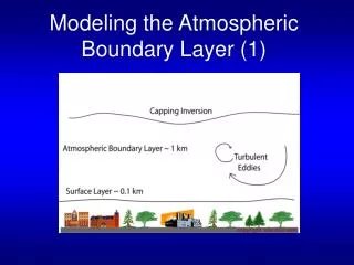
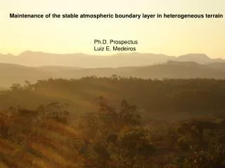
Maintenance of the stable atmospheric boundary layer in heterogeneous terrain Ph.D. ProspectusLuiz E. Medeiros
Outline • 1. Introduction – Background, relevance, and objectives of the proposed work • 2. Experimental data • 3. Plan of research • 4. Preliminary results • 5. Expected outcome • 6. Timeline
The Richardson number Bulk Richardson number Rib From: Pardyjak et al. 2002. BD Bulk Richardson number Rib SP Kinematic Heat Flux
The ‘conventional’ stable boundary layer From: Stull, R. B. 1988: An Introduction to Boundary Layer Meteorology, Kluwer Academic Publishers, 666pp. Momentum Flux Heat Flux From: Garratt, J. R., 1992: The atmospheric boundary layer, Cambridge, 316pp.
Wind tunnel study of bursting turbulence beneath a low level jet (Ohya et al., 2008) Re = 2800 w’ • Under stable conditions, turbulence can be intermittent and/or spatially localized if the terrain is not homogeneous. Ri Ricr = 0.25 Taylor transformation x = Ut
Motivation to better understand the SBL • Numerical weather prediction (NWP) models have difficulties to estimate surface minimum temperatures, height of the turbulent layer, and lifetime of low-pressure systems (low surface drag) [Viterbo et al. 1999; McCabe and Brown 2007]. • Models adopt the classical text book concept of continuous and horizontally homogeneous turbulence. Low level jet (LLJ) at the top of SBL, from where turbulence extracts energy. K-Theory - (Km and Kh) - stability functions in terms of bulk Richardson number Rib. • Different types of stability functions to adjust the amount of mixing: • no mixing when Rib > 1/4 – Short tails; • artificial mixing when Rib > 1/4 – Long tails. • Long tails better minimum temperature and more surface drag. • However, a too thick turbulent layer, LLJ too far from the ground and with weakened strength, weakened potential temperature inversion. • Spatial heterogeneity can be one of the reasons to justify unphysical extra mixing to occur. – Localized pockets of mixing attenuated by averaging process.
Field observation of the SBL and influences of the landscape • During nights with clear skies and weak pressure gradient over complex terrain, turbulence can be patchy and intermittent [Acevedo and Fitzjarrald 2003; Salmond and McKendry 2005]. St.1 St. 2 St. 3 St. 4 St. 5 St. 6 St. 8 St. 7 St. 9 St. 10
Field observation of the SBL and influences of the landscape • Intermittent turbulence - Breaking gravity waves, Kelvin-Helmholtz (K-H) shear instabilities, and density currents → flow instabilities → turbulence (Finnigan et al. 1984, Einaudi and Finnigan 1993; CASES -99 - Sun et al. 2004; Poulos et al. 2002.). LLJ is another possibility (Description adopted in textbooks- Garratt, J. R. 1992). • Land cover / land use, and topography are responsible for the positioning of “turbulent” and “stagnant” air layers. Representativeness of local measurements of wind, temperature, and other scalars are tied to these air layers.
Landscape and mixing From Acevedo and Fitzjarrald 2003. • LeMone et. al, 2003 - Rib >> 0.1 the flow close to the ground (~2m) can stay disconnected from the flow above; • Rib ~ 0.1 the flow close to the ground can stay connected to the flow aloft.- Froude Fr number and Rib,
Goals AF2003 FOG -82 • The goal of the proposed research is to establish a broader linkage between the observed flow with terrain surface characteristics and background flow under stable conditions. • We seek to understand better how the SBL develops over complex terrain. To do this we will map out the turbulence activity over a region with complex terrain and as well as to determine the horizontal and vertical extensions of air layers that compose the regional SBL.
1.1 Scientific Questions • Main question - How does the stable boundary layer form over complex terrain? • Follow–up questions (a) What is the role of topography and landscape structure in determining the representativeness of surface weather station measurements? (b) What is the relationship between nocturnal intermittent mixing events, and the mean thermodynamic, trace gas and dynamical structure of the SBL? (c) What method can be used to extrapolate surface fluxes that apply to a mesoscale area from a network of point measurements?
2. Data and model output 2.1. Hudson Valley Ambient Meteorology Study (HVAMS) 2.2. Harvard Forest Environmental Site (HF- EMS) 2.3. Large-scale Biosphere-Atmosphere experiment in Amazonia (LBA) 2.4. Mesoscale model simulations (UIB)
2.1. HVAMS • A long-term ASRC JRG observational program designed to understand the planetary boundary layer in the Hudson valley between the cities of Albany and Poughkeepsie.
HVAMS – Long Term Observational Period (LTOP) – From 11/02/03 to present time HOBO weather st. ASOS st. (ALB, POU) 4 → H1 S → H3 6 → H4 10_Anchor st. From Anchor st. we can build ensembles turbulence mixing events ~ 5 years of data. From all HOBOs too because we have ~ 4.5 years of data.
2.1. Land use and land cover map Resolution = 30m x 30m Same resolution topographic data. Source: USGS Global Land Information System http://gisdata.usgs.net/website/mrlc/viewr.html
2.2. Harvard Forest Environmental Measurement site (HF-EMS) 30m – Micromet Tower • 45 % red oak • 27 % red maple • 20 % hemlock • 6 % white ash (From: Staebler, 2003) This experiment started in 1989 and still running until the present time. It certainly has enough data to build ensembles about turbulence breakdowns.
2.4 Mesoscale model Meso-NH applied to HVAMS • Modeled output data for the IOP, obtained from the mesoscale model Meso-NH. Grid cell size 2km x 2km x 3m and time step 2s. • The simulations were performed by the meteorology research center of the Universitat de les Illes Balears (UIB), in Mallorca, Spain by Drs. Joan Cuxart and Maria Antonia Jiménez. Simulations are available for the nights of 06 – 07 and 07 – 08 of October, 2003 for comparison with surface observations and aircraft flight tracks. • Such data will serve us to investigate the formation of the cold air pool in the bottom of the Hudson valley, to estimate of radiative flux divergence across the SBL, and to understand channeling. [From: http://mesonh.aero.obs-mip.fr/mesonh/. A general description of the model operation is given by Lafore et al., (1998)]
Conceptual model • The valley topography channels the flow to be along-valley (southerly or northerly) inside the valley. • Turbulence breakdowns are likely to bring the wind direction at a particular station close to channeled direction (N or S). Whenever these events occur, they will be followed by downward momentum and heat fluxes. • We hypothesize that when there is a low level along-valley jet, and this jet is a main driver for breakdowns of turbulent intermittent events but is not the only mechanism for turbulence breakdowns. • As the night evolves, the valley floor fills up with cold air. This layer can slosh back and forth, introducing cross-valley motions beneath the jet, as cold air parcels from drainage flows try to adjust underneath it. Depending on constancy of the jet, and pooling of cold air, station can disconnect or connect .
Simulated q cross-section at mid-valley by Meso-NH 0900 UTC (0600 LT) October 8, 2003
Along valley flow felt at the surface (Wind roses obtained for the daytime period from September 19, 2003 until November 1, 2003.)
Along valley flow felt at the surface (Wind roses obtained for the nocturnal period from September 19, 2003 until November 1, 2003.)
Along valley flow above the surface on the night of 10/07/2003 – 10/08/2003 Aircraft and weather soundings UTC UTC SBL channeling CBL channeling
Schematic description of SBL interactions To address the scientific questions we start from the premise that the flow dynamics over a region is controlled by these external parameters: 25
Station 7 North Landscape: Agricultural clearance in a concave surface. West East 26 South Local landscape/Sheltering Wind rose and TF
Station 5 Landscape: Cherry orchard in convex surface.
3.1. Turbulence activity • To answer our scientific questions we first will separate periods in time series of wind and temperature by categories of standard deviation of the wind, or temperature or both combined (the flux product w’T’). • Standard deviation, , where x represents w’, T’ and w’T’. Guiding questions: 1 - Is the flow at the station connected or not the flow aloft (~ 100 to 150m above ground)? If not is it connected to other shallow flow like drainage? 2 – What is an intermittent event ?
3.1.1. Technique to identify intermittent events • Howell’s algorithm (Howell, 1994). • Originally the algorithm was designed to identify periods of abrupt changes in means of time series of any meteorological variables. • It was slightly changed to identify periods of abrupt changes in standard deviation. Time window = 60 min. Time window = 45 min.
Another tool - Wavelets October 13-14 2003 HVAMS flux product for station 1
2 - What is an intermittent event ? • Preliminary answer Due to the difficulties mentioned above to define intermittent events, will include the following conditions: • Wind speed, turbulence intensity (sigma-w), and potential temperature have to increase. • Wind direction has to align with the flow aloft (if turbulence is generated by shear instabilities caused be the LLJ). However, this condition has to be abandoned if the turbulence is generated by other mechanism. • All followed by downward momentum and heat fluxes.
Using simple weather stations to capture intermittent events and estimate fluxes • The idea of using HOBO weather stations to identify breakdowns of turbulent intermittent events consist on seeing if mutual increase in wind speed perturbation and temperature perturbation obtained 1min./data are related to increase in fluxes of momentum and heat. This idea will be tested (using flux stations during the IOP) by comparing minute averages of 1Hz or 10 Hz sonic data with direct flux measurements (Obtained from eddy-correlation technique). Ρcpσu’σT Heat flux (w/m^2) The following step will be to estimate the fluxes using this 1min./data through empirical relations like
3.2.1. Site representativeness – Importance of landscape features on the representativeness of local measurements • Guiding question: 1- What are the landscape characteristics of the sites that have more intense turbulent activity and as well the ones that have less? stable boundary layer: -low level jet; -size comparable to the; network size. stable surface layer: -local flows or low level jet; -when disconnected has smaller size than network size and when connect SBL size. • Observed wind, temperature, moisture, and other scalars are representative of certain volume of the atmosphere (air layer), but each time a mixing event happens it can bring “information” about these quantities from higher levels of the atmosphere.
3.2.2. Determining Land use / land cover and topography influences in the SBL dynamics in the Hudson valley • From the digital topographic map we aim to calculate the terrain slope and curvature in our study areas and compare it with wind directions associated to abrupt temperature changes. • The area of 3 km x 3 km (used for LU/LC map) are going to be the first attempt to correlate slope direction and wind direction, but if such relationships do not emerge, we will try larger and smaller areas.
3.2.2. Determining Land use / land cover and topography influences in the SBL dynamics in the Hudson valley • Through land use /land cover map we aim to establish a relationship with turbulent activity and minimum temperature. Hudson valley land cover / land use (Preliminary work completed.)
A plan to answer to question – 1 The fluxes calculations and counting of intermittent turbulent events will be done for all the 10 stations, and by doing so we will be able to find how the turbulence activity is distributed among the sites (i. e. which ones are more turbulent and less turbulent, and as well as more intermittent and less). In addition, if we have information about topography, land use / land cover, transmission factor, we can find what are the site characteristics in determining site exposure and turbulent activity. Correlations like: TF Vs. surface type (if we know the height and distance of the obstacles around a station we can determine its TF = exp(-kQobs) [Fujita and Wakimoto,1982]. TF Vs. turbulent activity.
3.3. Mesoscale influences • Guiding question 1- What is the relationship between turbulence activity and the external forcing (synoptic and/or mesoscale pressure gradient and cloud cover)? A plan to answer to question -1 We will correlate along-valley surface pressure gradient and cloud cover fraction to turbulence activity over a site and over the study region as well. Pressure data from the PAMs that had microbarometers during the IOP, and pressure data from the ASOS at Poughkeepsie and Albany during the LTOP will be used to calculate the surface pressure gradient. ASOS data at Albany and Poughkeepsie will provide the cloud cover fraction.
4. Preliminary results Aircraft/TB vertical soundings illustrate along-valley flow 30-31 October 2003
Night of October 30 - 31, 2003 Aircraft Profiles at 1B1 – Columbia County Aircraft Profiles at st. 4 - Green Acres Tethered balloon flying at constant height at st. 10 from 1700 LST until 0300 LST on October 16 -17, 2003
A close look at turbulent mixing on the case study night of October 30 – 31, 2003during IOP
October 30 – 31, 2003 Vertical velocity St. 2 St.1 St. 4 St. 3 St. 5 St. 6 St. 7 St. 8 St. 9 St. 10
October 30 – 31, 2003Wind speed St.1 St. 2 St. 4 St. 3 St. 6 St. 5 St. 7 St. 8 St. 9 St. 10
October 30 - 31, 2003Wind direction St.1 St. 2 St. 3 St. 4 St. 5 St. 6 St. 7 St. 8 St. 9 St. 10
October 30 – 31, 2003Momentum and heat fluxes St.1 St.1 St.1 St.1 St.1 St.1 St.1 St.1 St.1 St.1 St.1 St.1 St.1 St.1 St. 2 St. 2 St. 2 St. 2 St. 2 St. 2 St. 3 St. 3 St. 3 St. 3 St. 3 St. 3 St. 3 St. 3 St. 3 St. 3 St. 3 St. 3 St. 3 St. 4 St. 4 St. 4 St. 4 St. 4 St. 5 St. 5 St. 5 St. 5 St. 5 St. 5 St. 5 St. 5 St. 5 St. 5 St. 5 St. 6 St. 6 St. 6 St. 6 St. 7 St. 7 St. 7 St. 7 St. 7 St. 7 St. 7 St. 7 St. 7 St. 8 St. 8 St. 8 St. 9 St. 9 St. 9 St. 9 St. 9 St. 9 St. 9 St. 10 St. 10
Surface q October 30 – 31, 2003 Potential Temperature Thermal consequences of the intermittent mixing at the surface.
October 24 - 25No alignment of the wind at st. 7 with the SLLF W’ Wind speed wind direction Momentum and heat fluxes
Going back to the question - Is the flow at the station connected or not the flow aloft (~ 100 to 150m above ground)? If not is to connected to other shallow flow like drainage ? Preliminary answer If the wind direction at the station follows the wind direction of the flow aloft, the station is connect, if does not, is not. We will use the tethered balloon data to verify it during IOP and during LTOP Albany soundings. Bulk network properties (I) Used only 4 nights out of 45 (from IOP) + 4.5x365 (from LTOP) =1687 nights.
Bulk network properties (II) Scaled temperature envelope Vs. maximum network wind speed