Download
1 / 32
330 likes | 455 Views
This study explores the challenges of high-resolution satellite wind data observed during Hurricane Opal in October 1995. It addresses the negative impacts of observation errors, particularly spatial correlations, that distort data accuracy. The proposed solution, superobbing, averages wind data within 2º x 2º x 100 hPa boxes to create reduced-error superobservations, effectively thinning the dataset while retaining essential high-resolution information. Results indicate mixed outcomes across various regions, shedding light on the complex interplay of observation errors and future modeling improvements.

E N D
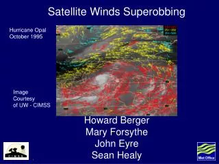
Satellite Winds Superobbing Hurricane Opal October 1995 Image Courtesy of UW - CIMSS Howard Berger Mary Forsythe John Eyre Sean Healy
Outline • Background/Problem • Superob Methodology • Method • Observation Error • Results • Conclusions/Future Work
Problem: • High - Resolution satellite wind data sets showed negative impact (Butterworth and Ingleby, 2000) Why? • Suspected that observations errors were spatially correlated • To account for this negative impact, wind data were/are thinned to 2º x 2º x 100 hPa boxes
Bormann et al. (2002) compared wind data to • co-located radiosondes showing statistically significant spatial error correlations up to 800 km. Met-7 W V NH Correlations Correlation Graphic from Bormann et al.2002
Question: Can we lower the data volume to reduce the effect of correlated error while making some use of the high-resolution data?
Proposed Solution: Average the observation - background (innovations) within a prescribed 3-d box to create a superobservation.
Advantages: • Data volume is reduced to same resolution that resulted from thinning. • Averaging removes some of the random, uncorrelated error within the data.
Superobbing Method:
1) Sort observations into 2º x 2º x 100 hPa boxes. 28 N 26 N 18 W 16 W
2) Within each box: Average u and v component innovations, latitude, longitude and pressures. 28 N 26 N 18 W 16 W
3) Find observation that is closest to average position and add averaged innovation to the background value at that observation location. 28 N 26 N 18 W 16 W
Superob Observation Error • Superobbing removes some of the random observation error. • This new error can be approximated by making a few assumptions about the errors within the background and the observation.
Superob Observation Error • Assume that within a box: • Observation and background errors not correlated with each other. • Background errors fully correlated. • Background errors have the same magnitude.
Superob Observation Error • Assumptions (cont): • All of the innovations weighted equally. • Constant observation error correlation.
Token Evil Math Slide Superob Observation Error Vector of Weights (1xN) Diagonal matrix of component observation errors (N x N) Observation Error Correlation Matrix (NxN)
Observation Correlation Matrix Correlation of ithobservation with jthobservation Correlation within box. Value calculated from correlation function in Bormann et al., 2002
00z 10 June, 2003. (20 N - 40 N) (0E 30 E) Old Observation Error Superob Error
Experimental Design • Control Run: • Operational Set up plus GOES BUFR VIS/IR/WV winds • GOES-9 is still Satob format • Thinning to 2˚ x 2˚ x 100 hPa boxes • Superob Experiment • Same as control run, except winds are superobbed to 2˚ x 2˚ x 100 hPa boxes
Experimental Design (cont) • Trial Period: 24 Jan -17 Feb 2004 • 4 Analyses and 6-hr forecasts • 00z,06z,12z,18z • 1 analysis and 5-day forecast (12z)
Token Model Info Slide • Grid – point model (288 E-W x 217 N-S) • Staggered Arakawa C-Grid • Approx 100 km horizontal resolution (one-half operational resolution) • 38 levels hybrid-eta configuration • 3D-Var Data Assimilation
Trial Statistics • % normalized root mean square (rms) error against control rms differences calculated for: • Mean sea-level pressure (PMSL) • 500 hPa height (H500) • 850 hPa wind (W850) • 250 hPa wind (W250) • In regions: • Northern Hemisphere (NH) • Tropics (TR) • Southern Hemisphere (SH) • For forecast periods of: • T+24, T+48, T+72 ,T+96 , T+120
TP – Observations TP – Analysis SH – Observations SH – Analysis NH – Observations NH – Analysis 4 3 2 Experiment – Control RMS Error (%) 1 0 -1 H500 T+24 H500 T+48 H500 T+72 H500 T+24 H500 T+48 H500 T+72 W250 T+24 W850 T+24 W850 T+48 W850 T+72 W250 T+24 W250 T+24 PMSL T+24 PMSL T+48 PMSL T+72 PMSL T+96 PMSL T+24 PMSL T+48 PMSL T+72 PMSL T+96 PMSL T+120 PMSL T+120 -2
Anomaly Correlations Vs. Forecast Range Compared to Analysis 500 hPa Height NH TR SH
T+24 Forecast – Sonde RMS Vector Error 250 hPa Wind NH TR SH
250 hPa u-component Analysis Increments
250 hPa u-component Analysis Increments
Results Summary • Superobbing experiment results are small and mixed • Generally more positive in the northern hemisphere than in the southern hemisphere or tropics • Time series results are mixed: Some forecasts better than control, some worse
Implications • Mixed results suggest either: • Random Error not most significant error component of AMVs • Superobbing set up not ideal to treat random error
Future Work • Back to basics approach • Re-calculate observation errors from innovation statistics • Experiment with “model independent” quality indicators and “model independent” components in Bufr file
Future Work (cont) • Stripped down impact experiment (i.e no ATOVS radiances) • Experiment using simulated AMV’s in Met Office System • Ideas from IWW!!!!!