Download
1 / 52
550 likes | 1.42k Views
Explore the concepts of deciles and percentiles in statistics, along with the five-number summary and coefficient of variation. Learn how to interpret data using box plots and shape measures like skewness and kurtosis. Discover the importance of summary statistics in real-life data analysis.

E N D
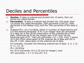
Deciles and Percentiles • Deciles: If data is ordered and divided into 10 parts, then cut points are called Deciles • Percentiles: If data is ordered and divided into 100 parts, then cut points are called Percentiles. 25th percentile is the Q1, 50th percentile is the Median (Q2) and the 75th percentile of the data is Q3. • Suppose PC= ((n+1)/100)p, where n=number of observations and p is the desired percentile. If PC is an integer than pth percentile of a data set is the (PC)th observation of the ordered set of that data. Otherwise let PI be the integer part of PC and f be the fractional part of PC. Then pth percentile= OI + (OII -OI)x`f where OI is the (PI)th observation of the ordered set of data and OII is the (PI +1)th observation of the ordered set of data. For example, Consider the following ordered set of data: 3, 5, 7, 8, 9, 11, 13, 15. PC= (9/100)p For 25 th percentile, PC=2.25 (not an integer), then 25th percentile = 5 + (7-5)x.25= 5.5
Coefficient of Variation • Coefficient of Variation: The standard deviation of data divided by it’s mean. It is usually expressed in percent. Coefficient of Variation=
Five Number Summary • Five Number Summary: The five number summary of a distribution consists of the smallest (Minimum) observation, the first quartile (Q1), the median(Q2), the third quartile, and the largest (Maximum) observation written in order from smallest to largest. • Box Plot: A box plot is a graph of the five number summary. The central box spans the quartiles. A line within the box marks the median. Lines extending above and below the box mark the smallest and the largest observations (i.e., the range). Outlying samples may be additionally plotted outside the range.
Boxplot Distribution of Age in Month
Side by Side Boxplot Trt 1 Trt 2 Trt 3
Choosing a Summary • The five number summary is usually better than the mean and standard deviation for describing a skewed distribution or a distribution with extreme outliers. The mean and standard deviation are reasonable for symmetric distributions that are free of outliers. • In real life we can’t always expect symmetry of the data. It’s a common practice to include number of observations (n), mean, median, standard deviation, and range as common for data summarization purpose. We can include other summary statistics like Q1, Q3, Coefficient of variation if it is considered to be important for describing data.
Shape of Data • Shape of data is measured by • Skewness • Kurtosis
Skewness • Measures of asymmetry of data • Positive or right skewed: Longer right tail • Negative or left skewed: Longer left tail
Kurtosis Kurtosis relates to the relative flatness or peakedness of a distribution. A standard normal distribution (blue line: µ = 0; = 1) has kurtosis = 0. A distribution like that illustrated with the red curve has kurtosis > 0 with a lower peak relative to its tails.
Brief concept of Statistical Softwares • There are many softwares to perform statistical analysis and visualization of data. Some of them are SAS (System for Statistical Analysis), S-plus, R, Matlab, Minitab, BMDP, Stata, SPSS, StatXact, Statistica, LISREL, JMP, GLIM, HIL, MS Excel etc. We will discuss MS Excel and SPSS in brief. • Some useful websites for more information of statistical softwares- http://www.galaxy.gmu.edu/papers/astr1.html http://ourworld.compuserve.com/homepages/Rainer_Wuerlaender/statsoft.htm#archiv http://www.R-project.org
Microsoft Excel • A Spreadsheet Application. It features calculation, graphing tools, pivot tables and a macro programming language called VBA (Visual Basic for Applications). • There are many versions of MS-Excel. Excel XP, Excel 2003, Excel 2007 are capable of performing a number of statistical analyses. • Starting MS Excel: Double click on the Microsoft Excel icon on the desktop or Click on Start --> Programs --> Microsoft Excel. • Worksheet: Consists of a multiple grid of cells with numbered rows down the page and alphabetically-tilted columns across the page. Each cell is referenced by its coordinates. For example, A3 is used to refer to the cell in column A and row 3. B10:B20 is used to refer to the range of cells in column B and rows 10 through 20.
Microsoft Excel Opening a document: File Open (From a existing workbook). Change the directory area or drive to look for file in other locations. Creating a new workbook: FileNewBlank Document Saving a File: FileSave Selecting more than one cell: Click on a cell e.g. A1), then hold the Shift key and click on another (e.g. D4) to select cells between and A1 and D4 or Click on a cell and drag the mouse across the desired range. • Creating Formulas: 1. Click the cell that you want to enter the formula, 2. Type = (an equal sign), 3. Click the Function Button, 4. Select the formula you want and step through the on-screen instructions.
Microsoft Excel • Entering Date and Time: Dates are stored as MM/DD/YYYY. No need to enter in that format. For example, Excel will recognize jan 9 or jan-9 as 1/9/2007 and jan 9, 1999 as 1/9/1999. To enter today’s date, press Ctrl and ; together. Use a or p to indicate am or pm. For example, 8:30 p is interpreted as 8:30 pm. To enter current time, press Ctrl and : together. • Copy and Paste all cells in a Sheet: Ctrl+A for selecting, Ctrl +C for copying and Ctrl+V for Pasting. • Sorting: Data Sort Sort By … • Descriptive Statistics and other Statistical methods: ToolsData Analysis Statistical method. If Data Analysis is not available then click on Tools Add-Ins and then select Analysis ToolPack and Analysis toolPack-Vba
Microsoft Excel Statistical and Mathematical Function: Start with ‘=‘ sign and then select function from function wizard Inserting a Chart: Click on Chart Wizard (or InsertChart), select chart, give, Input data range, Update the Chart options, and Select output range/ Worksheet. Importing Data in Excel: File open FileType Click on File Choose Option ( Delimited/Fixed Width) Choose Options (Tab/ Semicolon/ Comma/ Space/ Other) Finish. Limitations: Excel uses algorithms that are vulnerable to rounding and truncation errors and may produce inaccurate results in extreme cases.
Statistics Packagefor the Social Science (SPSS) A general purpose statistical package SPSS is widely used in the social sciences, particularly in sociology and psychology. SPSS can import data from almost any type of file to generate tabulated reports, plots of distributions and trends, descriptive statistics, and complex statistical analyzes. Starting SPSS: Double Click on SPSS on desktop or ProgramSPSS. Opening a SPSS file: FileOpen MENUS AND TOOLBARS Data Editor Various pull-down menus appear at the top of the Data Editor window. These pull-down menus are at the heart of using SPSSWIN. The Data Editor menu items (with some of the uses of the menu) are:
Statistics Packagefor the Social Science (SPSS) MENUS AND TOOLBARS FILE used to open and save data files EDIT used to copy and paste data values; used to find data in a file; insert variables and cases; OPTIONS allows the user to set general preferences as well as the setup for the Navigator, Charts, etc. VIEW user can change toolbars; value labels can be seen in cells instead of data values DATA select, sort or weight cases; merge files TRANSFORM Compute new variables, recode variables, etc.
Statistics Packagefor the Social Science (SPSS) • MENUS AND TOOLBARS ANALYZE perform various statistical procedures GRAPHS create bar and pie charts, etc UTILITIES add comments to accompany data file (and other, advanced features) ADD-ons these are features not currently installed (advanced statistical procedures) WINDOW switch between data, syntax and navigator windows HELP to access SPSSWIN Help information
Statistics Packagefor the Social Science (SPSS) MENUS AND TOOLBARS Navigator (Output) Menus When statistical procedures are run or charts are created, the output will appear in the Navigator window. The Navigator window contains many of the pull-down menus found in the Data Editor window. Some of the important menus in the Navigator window include: INSERT used to insert page breaks, titles, charts, etc. FORMAT for changing the alignment of a particular portion of the output
Statistics Packagefor the Social Science (SPSS) • Formatting Toolbar When a table has been created by a statistical procedure, the user can edit the table to create a desired look or add/delete information. Beginning with version 14.0, the user has a choice of editing the table in the Output or opening it in a separate Pivot Table (DEFINE!) window. Various pulldown menus are activated when the user double clicks on the table. These include: EDIT undo and redo a pivot, select a table or table body (e.g., to change the font) INSERT used to insert titles, captions and footnotes PIVOT used to perform a pivot of the row and column variables FORMAT various modifications can be made to tables and cells
Statistics Packagefor the Social Science (SPSS) • Additional menus CHART EDITOR used to edit a graph SYNTAX EDITOR used to edit the text in a syntax window • Show or hide a toolbar Click on VIEW ⇒ TOOLBARS ⇒ to show it/ to hide it • • Move a toolbar • Click on the toolbar (but not on one of the pushbuttons) and then drag the toolbar to its new location • • Customize a toolbar • Click on VIEW ⇒ TOOLBARS ⇒ CUSTOMIZE
Statistics Packagefor the Social Science (SPSS) Importing data from an EXCEL spreadsheet: Data from an Excel spreadsheet can be imported into SPSSWIN as follows: 1. In SPSSWIN click on FILE ⇒ OPEN ⇒ DATA. The OPEN DATA FILE Dialog Box will appear. 2. Locate the file of interest: Use the "Look In" pull-down list to identify the folder containing the Excel file of interest 3. From the FILE TYPE pull down menu select EXCEL (*.xls). 4. Click on the file name of interest and click on OPEN or simply double-click on the file name. 5. Keep the box checked that reads "Read variable names from the first row of data". This presumes that the first row of the Excel data file contains variable names in the first row. [If the data resided in a different worksheet in the Excel file, this would need to be entered.] 6. Click on OK. The Excel data file will now appear in the SPSSWIN Data Editor.
Statistics Packagefor the Social Science (SPSS) Importing data from an EXCEL spreadsheet: 7. The former EXCEL spreadsheet can now be saved as an SPSS file (FILE ⇒ SAVE AS) and is ready to be used in analyses. Typically, you would label variable and values, and define missing values. Importing an Access table SPSSWIN does not offer a direct import for Access tables. Therefore, we must follow these steps: 1. Open the Access file 2. Open the data table 3. Save the data as an Excel file 4. Follow the steps outlined in the data import from Excel Spreadsheet to SPSSWIN. Importing Text Files into SPSSWIN Text data points typically are separated (or “delimited”) by tabs or commas. Sometimes they can be of fixed format.
Statistics Packagefor the Social Science (SPSS) • Importing tab-delimited data In SPSSWIN click on FILE ⇒ OPEN ⇒ DATA. Look in the appropriate location for the text file. Then select “Text” from “Files of type”: Click on the file name and then click on “Open.” You will see the Text Import Wizard – step 1 of 6 dialog box. You will now have an SPSS data file containing the former tab-delimited data. You simply need to add variable and value labels and define missing values. • Exporting Data to Excel click on FILE ⇒ SAVE AS. Click on the File Name for the file to be exported. For the “Save as Type” select from the pull-down menu Excel (*.xls). You will notice the checkbox for “write variable names to spreadsheet.” Leave this checked as you will want the variable names to be in the first row of each column in the Excel spreadsheet. Finally, click on Save.
Statistics Packagefor the Social Science (SPSS) • Running the FREQUENCIES procedure 1. Open the data file (from the menus, click on FILE ⇒ OPEN ⇒ DATA) of interest. 2. From the menus, click on ANALYZE ⇒ DESCRIPTIVE STATISTICS ⇒ FREQUENCIES 3. The FREQUENCIES Dialog Box will appear. In the left-hand box will be a listing ("source variable list") of all the variables that have been defined in the data file. The first step is identifying the variable(s) for which you want to run a frequency analysis. Click on a variable name(s). Then click the [ > ] pushbutton. The variable name(s) will now appear in the VARIABLE[S]: box ("selected variable list"). Repeat these steps for each variable of interest. 4. If all that is being requested is a frequency table showing count, percentages (raw, adjusted and cumulative), then click on OK.
Statistics Packagefor the Social Science (SPSS) • Requesting STATISTICS Descriptive and summary STATISTICS can be requested for numeric variables. To request Statistics: 1. From the FREQUENCIES Dialog Box, click on the STATISTICS... pushbutton. 2. This will bring up the FREQUENCIES: STATISTICS Dialog Box. 3. The STATISTICS Dialog Box offers the user a variety of choices: • DESCRIPTIVES The DESCRIPTIVES procedure can be used to generate descriptive statistics (click on ANALYZE ⇒ DESCRIPTIVE STATISTICS ⇒ DESCRIPTIVES). The procedure offers many of the same statistics as the FREQUENCIES procedure, but without generating frequency analysis tables.
Statistics Packagefor the Social Science (SPSS) • Requesting CHARTS One can request a chart (graph) to be created for a variable or variables included in a FREQUENCIES procedure. 1. In the FREQUENCIES Dialog box click on CHARTS. 2. The FREQUENCIES: CHARTS Dialog box will appear. Choose the intended chart (e.g. Bar diagram, Pie chart, histogram. • Pasting charts into Word 1. Click on the chart. 2. Click on the pulldown menu EDIT ⇒ COPY OBJECTS 3. Go to the Word document in which the chart is to be embedded. Click on EDIT ⇒ PASTE SPECIAL 4. Select Formatted Text (RTF) and then click on OK 5. Enlarge the graph to a desired size by dragging one or more of the black squares along the perimeter (if the black squares are not visible, click once on the graph).
Statistics Packagefor the Social Science (SPSS) • BASIC STATISTICAL PROCEDURES: CROSSTABS 1. From the ANALYZE pull-down menu, click on DESCRIPTIVE STATISTICS ⇒ CROSSTABS. 2. The CROSSTABS Dialog Box will then open. 3. From the variable selection box on the left click on a variable you wish to designate as the Row variable. The values (codes) for the Row variable make up the rows of the crosstabs table. Click on the arrow (>) button for Row(s). Next, click on a different variable you wish to designate as the Column variable. The values (codes) for the Column variable make up the columns of the crosstabstable. Click on the arrow (>) button for Column(s). 4. You can specify more than one variable in the Row(s) and/or Column(s). A cross table will be generated for each combination of Row and Column variables
Statistics Packagefor the Social Science (SPSS) • Limitations: SPSS users have less control over data manipulation and statistical output than other statistical packages such as SAS, Stata etc. • SPSS is a good first statistical package to perform quantitative research in social science because it is easy to use and because it can be a good starting point to learn more advanced statistical packages.
Normal Distribution A density curve describes the overall pattern of a distribution. The total area under the curve is always 1. A distribution is normal if its density curve is symmetric, single-peaked and bell-shaped. Mean, Median, and mode are same for a normal distribution A normal distribution can be described if we know their mean and standard deviation. The probability density function of a normal variable with mean µ and standard deviation σ can be expressed as, Normality and independence of the data are two very important assumptions for most statistical methods
Normal Distribution If we know µ and σ, we know every thing about the normal distribution. Total area under the curve is 1 σ 2σ µ
Normal Distribution The 68-95-99.7 Rule In the normal distribution with mean µ and standard deviation σ: 68% of the observations fall within σ of the mean µ. 95% of the observations fall within 2σ of the mean µ. 99.7% of the observations fall within 3σ of the mean µ. σ σ 3σ 2σ 2σ 3σ
Normal Density Plot A sample of 100 observations from a normal distribution with mean 0 and standard deviation 1. 68% 95%
Normal Distribution Standardizing and z-Scores If x is an observation from a distribution that has mean µ and standard deviation σ, the standardized value of x is A standardized value is often called a z-score. If x is normal distribution with mean µ and standard deviation σ, then z is a standard normal variable with mean 0 and standard deviation 1.
Normal Distribution Let x1, x2, …., xn be n random variables each with mean µ and standard deviation σ, then sum of all of them ∑xi be also a normal with mean nµ and standard deviation σ√n. The distribution of mean is also a normal with mean µ and standard deviation σ/√n. The standardized score of the mean is, The mean of this standardized random variable is 0 and standard deviation is 1.
Assessing the normality of data • Most statistical methods assume that data are from a normal population. So it’s important to test the normality of the data. • Normal quantile plots If the points on a normal quantile plot lie close to diagonal line, the plot indicates that the data are normal. Otherwise, it indicates departure from normality. Points far away from the overall pattern indicates outliers. Minor wiggles can be overlooked. We will see normal quantile plots in next two slides. • Shapiro-Wilk W statistics, Kolmogorov-Smirnov (K-S) tests etc are being used for testing normality of the data. • To perform a K-S Test for Normality in SPSS, Analyze> Nonparametric Tests > 1 Sample K-S. Choose OK after selecting variable (s). • To perform Shapiro-Wilk test of normality in SAS use procedure ‘Univariate’.
Normal quantile plot q-q plot 100 sample observations from a normal distribution with mean 0 and standard deviation 1
Population and Sample • Population: The entire collection of individuals or measurements about which information is desired e.g. Average height of 5-year old children in USA. • Sample: A subset of the population selected for study. Primary objective is to create a subset of population whose center, spread and shape are as close as that of population. There are many methods of sampling. Random sampling, stratified sampling, systematic sampling, cluster sampling, multistage sampling, area sampling, qoata sampling etc. • Random Sample: A simple random sample of size n from a population is a subset of n elements from that population where the subset is chosen in such a way that every possible unit of population has the same chance of being selected. • Example: Consider a population of 5 numbers (1, 2, 3, 4, 5). How many random sample (without replacement) of size 2 can we draw from this population ? (1,2), (1,3), (1, 4), (1, 5), (2, 3), (2, 4), (2, 5), (3,4), (3,5), (4,5)
Population and Sample • Why do we need randomness in sampling? It reduces the possibility of subjective and other biases. Mean and variance of a random sample is an unbiased estimate of the population mean and variance respectively. • Population mean of the five numbers in previous slide is 3. Averages of 10 samples of sizes 2 are 1.5, 2, 2.5, 3, 2.5, 3, 3.5, 3.5, 4, 4.5. Mean of this 10 averages (1.5 +2 + 2.5 + 3 + 2.5 + 3+ 3.5+ 3.5+ 4+ 4.5)/10 =3 which is the same as the population mean.
Parameter and Statistic • Parameter: Any statistical characteristic of a population. Population mean, population median, population standard deviation are examples of parameters. • Statistic: Any statistical characteristic of a sample. Sample mean, sample median, sample standard deviation are some examples of statistics. • Statistical Issue: Describing population through census or making inference from sample by estimating the value of the parameter using statistic.
Census and Inference • Census: Complete enumeration of population units. • Statistical Inference: We sample the population (in a manner to ensure that the sample correctly represents the population) and then take measurements on our sample and infer (or generalize) back to the population. Example: We may want to know the average height of all adults (over 18 years old) in the U.S. Our population is then all adults over 18 years of age. If we were to census, we would measure every adult and then compute the average. By using statistics, we can take a random sample of adults over 18 years of age, measure their average height, and then infer that the average height of the total population is ``close to'' the average height of our sample.
Univariate, Bivariate, and Multivariate Data • Depending on how many variables we are measuring on the individuals or objects in our sample, we will have one of the three following types of data sets • Univariate: Measurements made on only one variable per observation. • Bivariate: Measurements made on two variables per observation. • Multivariate: Measurements made on more than two variables per observation.
Examining Relationship • Response Variable: Measures the outcome of the study, treatment, or experimental manipulation. • Explanatory Variable: Explains or influences changes in a response variable. This is also known as an independent variable or prediction variable. • Scatter plot: Shows the relationship between two quantitative variables measured on the same individuals. We look for the overall pattern and striking deviations from that pattern. Overall pattern of a scatter plot by the form, direction, and strength of the relationship. • Positive relation: Association in the same direction • Negative relation: Association in the opposite direction
Examining Relationship • Form: Linear relationship, Curve linear relationship, Cluster etc. • Linear Relationship: Points of the scatter plot show a straight-line pattern. • Strength of the Relationship is determined by how close the points in the scatter plot lie to a simple form such as line. • Correlation measures the strength between two variables. We will learn more about the relationship of variables later.
Proportion • Proportion: In many cases, it is appropriate to summarize a group of independent observations by the number of observations in the group that represent one of two outcomes. • Consider a variable X with two outcomes 1 and 0 for happening and not happening of some events correspondingly. Let p be the probability that the event happens then p=Prob(X=1). • Suppose, we want to estimate of the proportion of the Patients coming to duPont having some particular disease. To estimate this proportion (population), we need to take a sample of size n and examine if the patient is bearing that particular disease. Then the estimated proportion is,
Proportion • For large n, the sampling distribution of is approximately normal with mean P (Population Proportion) and the standard deviation • If probability of happening one event is p, then probability of not happening of the same event is 1-p and total probability is 1. • What is the difference between proportion and a sample mean? If X takes two values 0 or 1 and p is the proportion of happening an event i. e. p=prob(x=1), then proportion is the same as sample mean.
Binomial Distribution • Let us consider an experiment with two outcomes success (s) and failure (F) for each subject and the experiment was done for n subjects. The sequence of S and F can be arranged as follows- SSFSFFFSSFS……F where there are x success out of n trial. Then the probability distribution of x can written as The mean and variance of x are np and np(1-p).