Download
1 / 15
190 likes | 729 Views
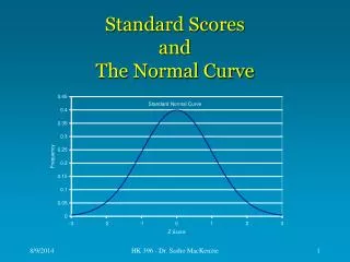
Percentiles and the Normal Curve. A Normal Curve. The Normal Approximation. Father’s Height. The height of the men in the sample was on average 69 inches; the SD was 3 inches. Estimate the percentage of these men with heights between 63 inches and 72 inches.

E N D
Father’s Height • The height of the men in the sample was on average 69 inches; the SD was 3 inches. • Estimate the percentage of these men with heights between 63 inches and 72 inches. • 63 inch = –2 SD; 72 inch = +1 SD. • The area between –2 and +1 is 47.5%, between 0 and +1 is 34.5%. • Approximately 82% of the men will be between 63 and 72 inches.
Financial Hardship • The average income for families was about $45,000. • The standard deviation was about $32,000. • The normal table tells us that 8% of the area lies to the left of –1.4 standard deviation. • This suggests that about 8% of the families have a negative income.
Percentiles • When the normal curve is not a good approximation to a histogram, we often use percentiles. • We have seen this idea before: the median is the 50th percentile. • The kth percentile is that number such that k percent of the data is less than that number.
Quartiles • The 25th percentile is often called the lower quartile. • The 75th percentile is often called the upper quartile. • The interquartile range is the 75th quartile – 25th quartile. • A ‘five number summary’ of a data set: minimum, lower quartile, median, upper quartile, maximum.
Percentiles and the Normal Curve • When a histogram does not follow the normal curve, we often use percentiles instead. • When a histogram does follow a normal curve, we can use the normal table to estimate the percentiles.
Example • Among all applicants to a university one year, the Math SAT scores averaged 535, the SD was 100, and the scores followed the normal curve. • Estimate the 95th percentile.
Example • This score is above average, by some number of standard deviations, z. • We cannot use the normal table directly, because this only gives us values for the area between –z and +z. • The area to the right of the z is 5%. Hence the area to the left of –z is 5%, too. The area between –z and +z is 90%.
Example • We can look this up in the normal table: z = 1.65. • You have to score 1.65 SD above average to be in the 95th percentile. • This is a score 1.65 x 100 = 165 points above average. • The 95th percentile of the score distribution is 535 + 165 = 700.
Percentile vs. Percentile Rank • A percentile on a test is a score: the 95th percentile is a score of 700. • A percentile rank is a percentile: if you score 700, then your percentile rank is 95%.
Freshman GPA • Suppose that the average freshmen GPA is around 3.0, and the SD is about 0.5. Assume that the histogram follows the normal curve. Estimate the GPA of someone in the 30th percentile. • This GPA is below average, say -z SD. • The area to the left is 30%. Thus, the area outside –z and z is 60%, inside 40%. • Look up in the table: z is between 0.5 and 0.55. • GPA is about 2.75.