Download
1 / 36
360 likes | 568 Views
Classification of Microarray data. Chris Holmes With thanks to: Jean Yang. Classification. Task: assign objects to classes (groups) on the basis of measurements made on the objects ( features) Unsupervised: classes unknown, want to discover them from the data (cluster analysis)

E N D
Classification of Microarray data Chris Holmes With thanks to: Jean Yang
Classification • Task: assign objects to classes (groups) on the basis of measurements made on the objects (features) • Unsupervised: classes unknown, want to discover them from the data (cluster analysis) • Supervised (classification/discrimination): class labels are predefined, want to use a (training or learning) set of labeled objects to form a classifier for classification of future observations, and to learn about discriminative features
Basic principles of classification • Each object has an associated class label (or response) Y {1, 2, …, K} and a feature vector (vector of predictor variables) of G measurements: X = (X1, …, XG) • Aim:predict Y from X and learn about influence of (X1, …, XG) Predefined Class {1,2,…K} K 1 2 Objects Y = Class Label = 2 X = Feature vector {colour, shape} Classification rule ? X = {red, square} Y = ?
Classification Learning Set Data with known classes Prediction Classification rule Data with unknown classes Classification Technique Class Assignment Discrimination
Learning set Bad prognosis recurrence < 5yrs Good Prognosis recurrence > 5yrs ? Good Prognosis Matesis > 5 Predefine classes Clinical outcome Objects Array Feature vectors Gene expression new array Reference L van’t Veer et al (2002) Gene expression profiling predicts clinical outcome of breast cancer. Nature, Jan. . Classification rule
Learning set Predefine classes Tumor type B-ALL T-ALL AML T-ALL ? Objects Array Feature vectors Gene expression new array Reference Golub et al (1999) Molecular classification of cancer: class discovery and class prediction by gene expression monitoring. Science 286(5439): 531-537. Classification Rule
Parameter Estimation • Almost all classification models have a number of free parameters that are “learnt” (assigned values) using the training set of examples. • Question: given a data set, how do we find an optimal set of parameter values? • Two components: • A cost function; that defines how good a particular parameter value is • A search strategy; to search over parameter space and return the parameter values with lowest cost
Classification rule Maximum likelihood discriminant rule • A maximum likelihood estimator (MLE) chooses the parameter value that makes the chance of the observations the highest • For known class conditional densities pk(X), the maximum likelihood (ML)discriminant rule predicts the class of an observationX by C(X) = argmaxk pk(X)
Gaussian ML discriminant rules • For multivariate Gaussian (normal) class densities X|Y= k ~ N(k, k), the ML classifier is C(X) = argmink {(X - k) k-1(X - k)’ + log| k |} • In general, this is a quadratic rule (Quadratic discriminant analysis, or QDA) • In practice, population mean vectors k and covariance matrices k are estimated by corresponding sample quantities
ML discriminant rules - special cases [DLDA] Diagonal linear discriminant analysis class densities have the same diagonal covariance matrix = diag(s12, …, sp2) [DQDA] Diagonal quadratic discriminant analysis) class densities have different diagonal covariance matrix k= diag(s1k2, …, spk2) Note. Weighted gene voting of Golub et al. (1999) is a minor variant of DLDA for two classes (wrong variance calculation).
Nearest neighbor classification • Based on a measure of distance between observations (e.g. Euclidean distance or one minus correlation). • k-nearest neighbor rule (Fix and Hodges (1951)) classifies an observation X as follows: • find thek observations in the learning set closest to X • predict the class of X by majority vote, i.e., choose the class that is most common among those k observations. • The number of neighbors kcan be chosen by cross-validation (more on this later).
Classification tree • Partition the feature space into a set of rectangles, then fit a simple model in each one • Binary tree structured classifiers are constructed by repeated splits of subsets (nodes) of the measurement space X into two descendant subsets (starting with X itself) • Each terminal subset is assigned a class label; the resulting partition of X corresponds to the classifier
Gene 1 Mi1 < -0.67 yes no Gene 2 Mi2 > 0.18 2 yes no 0 1 Classification tree Gene 2 0 2 0.18 Gene 1 1 -0.67
Three aspects of tree construction • Split selection rule: • Example, at each node, choose split maximizing decrease in impurity (e.g.Gini index, entropy, misclassification error). • Split-stopping: • Example, grow large tree, prune to obtain a sequence of subtrees, then use cross-validation to identify the subtree with lowest misclassification rate. • Class assignment: • Example, for each terminal node, choose the class minimizing the resubstitution estimate of misclassification probability, given that a case falls into this node.
Other classifiers include… • Neural networks • Logistic regression • Projection pursuit • Bayesian belief networks
Why select features? Top 100 feature selection Selection based on variance No feature selection Correlation plot Data: Leukemia, 3 class +1 -1
Explicit feature selection • One-gene-at-a-time approaches. Genes are ranked based on the value of a univariate test statistic such as: t- or F-statistic or their non-parametric variants (Wilcoxon/Kruskal-Wallis); p-value. • Possible meta-parameters include the number of genes G or a p-value cut-off. A formal choice of these parameters may be achieved by cross-validation or bootstrap procedures. • Multivariate approaches. More refined feature selection procedures consider the joint distribution of the expression measures, in order to detect genes with weak main effects but possibly strong interaction. • Bo & Jonassen (2002): Subset selection procedures for screening gene pairs to be used in classification. • Breiman (1999): ranks genes according to importance statistic define in terms of prediction accuracy. Note that tree building itself does not involve explicit feature selection.
Implicit feature selection • Feature selection may also be performed implicitly by the classification rule itself. • In classification trees, features are selected at each step based on reduction in impurity and The number of features used (or size of the tree) is determined by pruning the tree using cross-validation. Thus, feature selection is inherent part of tree-building and pruning deals with over-fitting. • Shrinkage methods and adaptive distance function. May be used for LDA and kNN.
Performance assessment • Any classification model needs to be evaluated for its performance on the future samples. It is almost never the case in microarray studies that a large independent population-based collection of samples is available at the time of initial classifier-building phase. • One needs to estimate future performance based on what is available: often the same set that is used to build the classifier. • Assessing performance of the classifier based on • Cross-validation. • Test set • Independent testing on future dataset
Diagram of performance assessment Classifier Training Set Resubstitution estimation Training set Performance assessment Test set estimation Classifier Independent test set
Performance assessment (I) • Resubstitution estimation: error rate on the learning set. • Problem: downward bias • Test set estimation: 1) divide learning set into two sub-sets, L and T; Build the classifier on L and compute the error rate on T. 2) Build the classifier on the training set (L) and compute the error rate on an independent test set (T). • L and T must be independent and identically distributed (i.i.d). • Problem: reduced effective sample size
Diagram of performance assessment Classifier Training Set Resubstitution estimation (CV) Learning set Cross Validation Classifier Training set Performance assessment (CV) Test set Test set estimation Classifier Independent test set
Performance assessment (II) • V-fold cross-validation (CV) estimation: Cases in learning set randomly divided into V subsets of (nearly) equal size. Build classifiers by leaving one set out; compute test set error rates on the left out set and averaged. • Bias-variance tradeoff: smaller V can give larger bias but smaller variance • Computationally intensive. • Leave-one-out cross validation (LOOCV). (Special case for V=n). Works well for stable classifiers (k-NN, LOOCV)
Performance assessment (III) • Common practice to do feature selection using the learning , then CV only for model building and classification. • However, usually features are unknown and the intended inference includes feature selection. Then, CV estimates as above tend to be downward biased. • Features (variables) should be selected only from the learning set used to build the model (and not the entire set)
Another component in classification rule:aggregating classifiers Classifier 1 Resample 1 Classifier 2 Resample 2 Training Set X1, X2, … X100 Aggregate classifier Classifier 499 Resample 499 Examples: Bagging Boosting Random Forest Classifier 500 Resample 500
Aggregating classifiers:Bagging Test sample Resample 1 X*1, X*2, … X*100 Tree 1 Class 1 Resample 2 X*1, X*2, … X*100 Tree 2 Class 2 Training Set (arrays) X1, X2, … X100 Lets the tree vote 90% Class 1 10% Class 2 Resample 499 X*1, X*2, … X*100 Tree 499 Class 1 Resample 500 X*1, X*2, … X*100 Tree 500 Class 1
Comparison study • Leukemia data – Golub et al. (1999) • n = 72 samples, • G = 3,571 genes, • 3 classes (B-cell ALL, T-cell ALL, AML). • Reference: S. Dudoit, J. Fridlyand, and T. P. Speed (2002). Comparison of discrimination methods for the classification of tumors using gene expression data. Journal of the American Statistical Association, Vol. 97, No. 457, p. 77-87
Leukemia data, 3 classes: Test set error rates;150 LS/TS runs
Results • In the main comparison, NN and DLDA had the smallest error rates. • Aggregation improved the performance of CART classifiers. • For the leukemia datasets, increasing the number of genes to G=200 didn't greatly affect the performance of the various classifiers.
Comparison study – discussion (I) • “Diagonal” LDA: ignoring correlation between genes helped here. Unlike classification trees and nearest neighbors, DLDA is unable to take into account gene interactions. • Classification trees are capable of handling and revealing interactions between variables. In addition, they have useful by-product of aggregated classifiers: prediction votes, variable importance statistics. • Although nearest neighbors are simple and intuitive classifiers, their main limitation is that they give very little insight into mechanisms underlying the class distinctions.
Summary (I) • Bias-variance trade-off. Simple classifiers do well on small datasets. As the number of samples increases, we expect to see that classifiers capable of considering higher-order interactions (and aggregated classifiers) will have an edge. • Cross-validation . It is of utmost importance to cross-validate for every parameter that has been chosen based on the data, including meta-parameters • what and how many features • how many neighbors • pooled or unpooled variance • classifier itself. If this is not done, it is possible to wrongly declare having discrimination power when there is none.
Summary (II) • Generalization error rate estimation. It is necessary to keep sampling scheme in mind. • Thousands and thousands of independent samples from variety of sources are needed to be able to address the true performance of the classifier. • We are not at that point yet with microarrays studies. Van Veer et al (2002) study is probably the only study to date with ~300 test samples.
Bad Good Case studies Learning set Classification Rule Reference 1 Retrospective study L van’t Veer et al Gene expression profiling predicts clinical outcome of breast cancer. Nature, Jan 2002. . Feature selection. Correlation with class labels, very similar to t-test. Using cross validation to select 70 genes Reference 2 Retrospective study M Van de Vijver et al. A gene expression signature as a predictor of survival in breast cancer. The New England Jouranl of Medicine, Dec 2002. 295 samples selected from Netherland Cancer Institute tissue bank (1984 – 1995). Results” Gene expression profile is a more powerful predictor then standard systems based on clinical and histologic criteria • Agendia (formed by reseachers from the Netherlands Cancer Institute) • Plan to start in Oct, 2003 • 3000 subjects [Health Council of the Netherlands] • 5000 subjects New York based Avon Foundation. • Custorm arrays are made by Aglient including • 70 genes + 1000 controls Reference 3 Prospective trials. Aug 2003 Clinical trials http://www.agendia.com/
Jean Yee Hwa Yang, University of California, San Francisco, http://www.biostat.ucsf.edu/jean/ Acknowledgements