Microarray Classification
Microarray Classification. Xiaole Shirley Liu STAT115/STAT215. Microarray Classification. ?. Classification. Equivalent to machine learning methods Task: assign object to class based on measurements on object E.g. is sample normal or cancer based on expression profile?


Microarray Classification
E N D
Presentation Transcript
Microarray Classification Xiaole Shirley Liu STAT115/STAT215
Classification • Equivalent to machine learning methods • Task: assign object to class based on measurements on object • E.g. is sample normal or cancer based on expression profile? • Unsupervised learning • Ignore known class labels • Sometimes can’t separate even the known classes • Supervised learning: • Extract useful features based on known class labels to best separate classes • Can over fit the data, so need to separate training and test set
Clustering Classification • Which known samples does the unknown sample cluster with? • No guarantee that the known sample will cluster • Try batch removal or different clustering methods • Change linkage, select subset genes (semi-supervised)
K Nearest Neighbor • Used in missing value estimation • For observation X with unknown label, find the K observations in the training data closest (e.g. correlation) to X • Predict the label of X based on majority vote by KNN • K can be determined by predictability of known samples, semi-supervised again!
KNN Example • Can extend KNN by assigning weights to the neighbors by inverse distance from the test-sample • Offer little insights into mechanism
Dimension Reduction • High dimensional data points are difficult to visualize • Always good to plot data in 2D or 3 D • Easier to detect or confirm the relationship among data points • Catch stupid mistakes (e.g. in clustering) • Two ways to reduce: • By genes: some genes are similar or have little information • By samples: some experiments are similar or have little information
Dimension Reduction • Techniques • MDS, PCA, LDA, all fit for classification • MDS: multidimensional scaling • Based on distance between data in high dimensional space (e.g. correlations) • Give 2-3D representation approximating the pairwise distance relationship as much as possible • Non-linear projection
Principal Component Analysis • Linear transformation that projects the data on to new coordinate system (linear combinations of the original variables) to capture as much of the variation in data as possible • The first principal component accounts for the greatest possible variance in dataset • The second principal component accounts for the next highest variance and is uncorrelated with (orthogonal to) the first principal component.
Finding the Projections • Looking for a linear combination to transform the original data matrix X to: Y= TX=1 X1+ 2 X2+..+ p Xp • Where =(1 , 2 ,.., p)Tis a column vector of weights with 1²+ 2²+..+ p²=1 • Maximize the variance of the projection of the observations on the Y variables
Finding the Projections Good Better • The direction of isgiven by the eigenvector1correponding to the largesteigenvalue of matrix C • The second vectorthatis orthogonal (uncorrelated) to the first is the one that has the second highest variance whichcomes to be the eignevectorcorresponding to the second eigenvalue
Principal Component Analysis • Achieved by singular value decomposition (SVD): X = UDVT • X is the original data • U is the relative projection of the points • V is project directions • v1 is direction of the first projection • Linear combination (relative importance) of each gene if PCA on samples
PCA • D is scaling factor (eigenvalue) • Diagonal matrix, d1 d2 d3 … 0 • Measures the variances captures by the mth principal component • u1d1 is distance along v1 from origin (first principal components) • Expression value projected on v1 • v2is 2nd projection direction, u2d2 is 2nd principal component, so on
PCA Example Blood transcriptome of healthy individual (HI), cardiovascular risk factor individuals (RF), individuals with asymptomatic left ventricular dysfunction groups (ALVD) and chronic heart failure patients (CHF).
Interpretation of components • See the weightsof variables in each component • If Y1= 0.89 X1 +0.15X2 -0.77X3+0.51X4 • ThenX1 and X3have the highestweightsand so are the mostimportant variable in the first PC, offerssomebiological insights • PCA isonlypowerful if the biological question isrelated to the highest variance in the dataset • PCA is a good clusteringmethod, and canbeconducted on genes or on samples
Supervised Learning Performance Assessment • If error rate is estimated from whole learning data set, could overfit the data (do well now, but poorly in future observations) • Divide observations into L1 and L2 • Build classifier using L1 • Compute classifier error rate using L2 • Requirement: L1 and L2 are iid (independent & identically-distributed) • N-fold cross validation • Divide data into N subset (equal size), build classifier on (N-1) subsets, compute error rate on left out subset
Fisher’s Linear Discriminant Analysis • First collect differentially expressed genes • Find linear projection so as to maximize class separability (b/t to w/i group sum of sq) • Can be used for dimension reduction as well
LDA • 1D, find two group means, cut at midpoint • 2D, connect two group means with line, use a line orthogonal to the connecting line and pass through the center • Limitation: • Does not consider non-linear relationship • Assume class mean capture most of information • Weighted voting: variation of LDA • Informative genes given different weight based on how informative it is at classifying samples (e.g. t-statistic)
Logistic Regression • Data: (yi, xi), i=1,…, n; (binary responses). • Predict the odds of being a case based on the values of the independent variables (predictors) • In practice, one estimates the ’s using the training data. (can use R) • The decision boundary is determined by the linear regression, i.e., classify yi =1 if Model:
LDA vs Logistic Regression • If assumptions are correct, LDA tends to estimate parameters more efficiently • LDA is not robust to outliers • Logistic regression relies on fewer assumptions, so tends to be more robust • In practice LDA and logistic regression often give similar results
Classification And Regression Tree • Split data using set of binary (or multiple value) decisions • Root node (all data) has certain impurities, need to split the data to reduce impurities
CART • Measure of impurities • Entropy • Gini index impurity • Example with Gini: multiply impurity by number of samples in the node • Root node (e.g. 8 normal & 14 cancer) • Try split by gene xi (xi 0, 13 cancer; xi< 0, 1 cancer & 8 normal): • Split at gene with the biggest reduction in impurities
CART • Assume independence of partitions, same level may split on different gene • Stop splitting • When impurity is small enough • When number of node is small • Pruning to reduce over fit • Training set to split, test set for pruning • Split has cost, compared to gain at each split
Support Vector Machine • SVM • Which hyperplane is the best?
Support Vector Machine • SVM finds the hyperplane that maximizes the margin • Margin determined by support vectors (samples lie on the class edge), others irrelevant
Support Vector Machine • SVM finds the hyperplane that maximizes the margin • Margin determined by support vectors others irrelevant • Extensions: • Soft edge, support vectors diff weight • Non separable: slack var > 0 Max (margin – # bad)
Nonlinear SVM • Project the data through higher dimensional space with kernel function, so classes can be separated by hyperplane • A few implemented kernel functions available in Matlab & BioConductor, the choice is usually trial and error and personal experience K(x,y) = (xy)2
Outline • Dimension reduction techniques • MDS, PCA, LDA • Unsupervised learning method • Clustering, KNN, MDS • PCA • Supervised learning for classification • LDA, logistic regression • CART, SVM • Importance of cross validation