Introduction to Classification Issues in Microarray Data Analysis
Introduction to Classification Issues in Microarray Data Analysis. Jane Fridlyand Jean Yee Hwa Yang University of California, San Francisco Elsinore, Denmark May 17-21, 2004. Brief Overview of the Life-Cycle. Life Cycle. Biological question. Experimental design. Failed.

Introduction to Classification Issues in Microarray Data Analysis
E N D
Presentation Transcript
Introduction to Classification Issues in Microarray Data Analysis Jane Fridlyand Jean Yee Hwa Yang University of California, San Francisco Elsinore, Denmark May 17-21, 2004
Life Cycle Biological question Experimental design Failed Microarray experiment Quality measurement Image analysis Pre-processing Pass Analysis Clustering Discrimination Estimation Testing Biological verification and interpretation
The steps outlined in the “Life Cycle” need to be carefully thought through and re-adjusted for each data type/platform combination. Experimental design will impact what questions should be asked and may be answered once the data are collected. • To call in the statistician after the experiment is done may be no more than asking him to perform a postmortem examination: he may be able to say what the experiment died of. Sir RA Fisher
* * * * * SAGE Nylon membrane Different Technologies GeneChipAffymetrix Illumina Bead Array cDNA microarray Agilent: Long oligo Ink Jet CGH
Some statistical issues • Designing gene expression experiments. • Acquiring the raw data: image analysis. • Assessing the quality of the data. • Summarizing and removing artifacts from the data. • Interpretation and analysis of the data: • Discovering which genes are differentially expressed • Discovering which genes exhibit interesting expression patterns • Detection of gene regulatory mechanisms. • and many others.. For a review see Smyth, Yang and Speed, “Statistical issues in microarray data analysis”, In: Functional Genomics: Methods and Protocols, Methods in Molecular Biology, Humana Press, March 2003 Lots of other bioinformatics issues …
Image analysis CEL, CDF files gpr, gal files UCSF spot file • Short-oligonucleotide chip data: • quality assessment, • background correction, • probe-level normalization, • probe set summary • Two-color spotted array data: • quality assessment; diagnostic plots, • background correction, • array normalization. • Array CGH data: • quality assessment; diagnostic plots, • , background correction • clones summary; • array normalization. Quality assessment Pre-processing probes by sample matrix of log-ratios or log-intensities • Analysis of expression data: • Identify D.E. genes, estimation and testing, • clustering, and • discrimination. Analysis
Linear Models • Examples • Identify differential expression genes among two or more tumor subtypes or different cell treatments. • Look for genes that have different time profiles between different mutants. • Looking for genes associated with survival. Linear Models Specific examples T-tests F-tests Empirical bayes SAM
Examples • We can cluster cell samples(cols), • the identification of new/unknown tumor sub classes or cell sub types using gene expression profiles. • We can cluster genes (rows) , • using large numbers of yeast experiments, to identify groups of co-expressed genes. Clustering • Algorithms • Hierarchical clustering • Self-organizing maps • Partition around medoids (pam)
Gene 1 Mi1 < -0.67 yes no Gene 2 Mi2 > 0.18 AML yes no B-ALL T-ALL Learning set Discrimination B-ALL T-ALL AML ? • Questions • Identification of groups of genes that predictive of a particular class of tumors? • Can I use the expression profile of cancer patients to predict survival? • Classification rules • DLDA or DQDA • k-nearest neighbor (knn) • Support vector machine (svm) • Classification tree
Annotation Nucleotide Sequence TCGTTCCATTTTTCTTTAGGGGGTCTTTCCCCGTCTTGGGGGGGAGGAAAAGTTCTGCTGCCCTGATTATGAACTCTATAATAGAGTATATAGCTTTTGTACCTTTTTTACAGGAAGGTGCTTTCTGTAATCATGTGATGTATATTAAACTTTTTATAAAAGTTAACATTTTGCATAAT AAACCATTTTTG GenBank accession AV128498 Riken ID ZX00049O01 Locuslink 15903 MGD MGI:96398 Name Inhibitor of DNA binding 3 UniGene Mm.110 Gene Symbol Idb3 Map Position Chromosome:4 66.0 cM Literature Swiss-Prot P20109 GO GO:0000122 GO:0005634 GO:0019904 Bay Genomics ES cells Biochemical pathways (KEGG) PubMed12858547 2000388 etc
What is your questions? • What are the targets genes for my knock-out gene? • Look for genes that have different time profiles between different cell types. Gene discovery, differential expression • Is a specified group of genes all up-regulated in a specified conditions? Gene set, differential expression • Can I use the expression profile of cancer patients to predict survival? • Identification of groups of genes that predictive of a particular class of tumors? Class prediction, classification • Are there tumor sub-types not previously identified? • Are there groups of co-expressed genes? Class discovery, clustering • Detection of gene regulatory mechanisms. • Do my genes group into previously undiscovered pathways? Clustering. Often expression data alone is not enough, need to incorporate sequence and other information
cDNA gene expression data Data on G genes for n samples mRNA samples sample1 sample2 sample3 sample4 sample5 … 1 0.46 0.30 0.80 1.51 0.90 ... 2 -0.10 0.49 0.24 0.06 0.46 ... 3 0.15 0.74 0.04 0.10 0.20 ... 4 -0.45 -1.03 -0.79 -0.56 -0.32 ... 5 -0.06 1.06 1.35 1.09 -1.09 ... Genes Gene expression level of gene i in mRNA samplej = (normalized) Log(Red intensity / Green intensity)
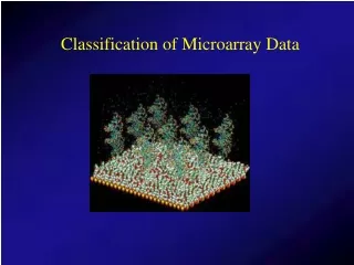
Classification • Task: assign objects to classes (groups) on the basis of measurements made on the objects • Unsupervised: classes unknown, want to discover them from the data (cluster analysis) • Supervised: classes are predefined, want to use a (training or learning) set of labeled objects to form a classifier for classification of future observations
Example: Tumor Classification • Reliable and precise classification essential for successful cancer treatment • Current methods for classifying human malignancies rely on a variety of morphological, clinical and molecular variables • Uncertainties in diagnosis remain; likely that existing classes are heterogeneous • Characterize molecular variations among tumors by monitoring gene expression (microarray) • Hope: that microarrays will lead to more reliable tumor classification (and therefore more appropriate treatments and better outcomes)
Tumor Classification Using Gene Expression Data Three main types of statistical problems associated with tumor classification: • Identification of new/unknown tumor classes using gene expression profiles (unsupervised learning – clustering) • Classification of malignancies into known classes (supervised learning – discrimination) • Identification of “marker” genes that characterize the different tumor classes (feature or variable selection).
Generic Clustering Tasks • Estimating number of clusters • Assigning each object to a cluster • Assessing strength/confidence of cluster assignments for individual objects • Assessing cluster homogeneity
What to cluster • Samples: To discover novel subtypes of the existing groups or entirely new partitions. Their utility needs to be confirmed with other types of data, e.g. clinical information. • Genes: To discover groups of co-regulated genes/ESTs and use these groups to infer function where it is unknown using members of the groups with known function.
Basic principles of clustering Aim: to group observations or variables that are “similar” based on predefined criteria. Issues: Which genes / arrays to use? Which similarity or dissimilarity measure? Which method to use to join clusters/observations? Which clustering algorithm? How to validate the resulting clusters? It is advisable to reduce the number of genes from the full set to some more manageable number, before clustering. The basis for this reduction is usually quite context specific and varies depending on what is being clustered, genes or arrays.
Clustering of genes Array Data For each gene, calculate a summary statistics and/or adjusted p-values Biological verification Set of candidate DE genes. Similarity metrics Descriptive interpretation Clustering Clustering algorithm
Clustering of samples and genes Array Data Set of samples to cluster Set of genes to use in clustering (DO NOT use class labels in the set determination). Similarity metrics Descriptive Interpretation of genes separating novel subgroups of the samples Clustering algorithm Clustering Validation of clusters with clinical data
Which similarity or dissimilarity measure? • A metric is a measure of the similarity or dissimilarity between two data objects • Two main classes of metric: • Correlation coefficients (similarity) • Compares shape of expression curves • Types of correlation: • Centered. • Un-centered. • Rank-correlation • Distance metrics (dissimilarity) • City Block (Manhattan) distance • Euclidean distance
Correlation (a measure between -1 and 1) • Pearson Correlation Coefficient (centered correlation) Sx = Standard deviation of x Sy = Standard deviation of y • Others include Spearman’s and Kendall’s You can use absolute correlation to capture both positive and negative correlation Positive correlation Negative correlation
Potentialpitfalls Correlation = 1
City Block (Manhattan) distance: Sum of differences across dimensions Less sensitive to outliers Diamond shaped clusters Euclidean distance: Most commonly used distance Sphere shaped cluster Corresponds to the geometric distance into the multidimensional space Y Condition 2 X Condition 1 Distance metrics Y Condition 2 X Condition 1 where gene X = (x1,…,xn) and gene Y=(y1,…,yn)
Euclidean vs Correlation (I) • Euclidean distance • Correlation
How to Compute Group Similarity? Four Popular Methods: • Given two groups g1 and g2, • Single-link algorithm: s(g1,g2)= similarity of the closest pair • Complete-link algorithm: s(g1,g2)= similarity of the farthest pair • Average-link algorithm: s(g1,g2)= average of similarity of all pairs • Centroid algorithm: s(g1,g2)= distance between centroids of the two clusters
Distance between clustersExamples of clustering methods Single (nearest neighbor) Leads to the “cluster chains” Complete (furtherest neighbor): Leads to small compact clusters x x Average (Mean) linkage Distance between centroids
Comparison of the Three Methods • Single-link • “Loose” clusters • Individual decision, sensitive to outliers • Complete-link • “Tight” clusters • Individual decision, sensitive to outliers • Average-link or centroid • “In between” • Group decision, insensitive to outliers • Which one is the best? Depends on what you need!
Clustering algorithms • Clustering algorithm comes in 2 basic flavors Hierarchical Partitioning
Partitioning methods • Partition the data into a pre-specified number k of mutually exclusive and exhaustive groups. • Iteratively reallocate the observations to clusters until some criterion is met, e.g. minimize within cluster sums of squares. Ideally, dissimilarity between clusters will be maximized while it is minimized within clusters. • Examples: • k-means, self-organizing maps (SOM), PAM, etc.; • Fuzzy (each object is assigned probability of being in a cluster): needs stochastic model, e.g. Gaussian mixtures.
Partitioning methods K = 2
Partitioning methods K = 4
Example of a partitioning algorithm K-Means or PAM (Partitioning Around Medoids) • Given a similarity function • Start with k randomly selected data points • Assume they are the centroids (medoids) of k clusters • Assign every data point to a cluster whose centroid (medoid) is the closest to the data point • Recompute the centroid (medoid) for each cluster • Repeat this process until the similarity-based objective function converges
Mixture Model for Clustering P(X|Cluster1) P(X|Cluster2) P(X|Cluster3) P(X)=1P(X|Cluster1)+ 2P(X|Cluster2)+3P(X|Cluster3)
Mixture Model Estimation • Likelihood function (generally Gaussian) • Parameters: e.g., i, i, I • Using EM algorithm • Similar to “soft” K-mean • Number of clusters can be determined using a model-selection criterion, e.g. BIC (Raftery and Fraley, 1998)
Hierarchical methods • Hierarchical clustering methods produce a tree or dendrogram. • They avoid specifying how many clusters are appropriate by providing a partition for each k obtained from cutting the tree at some level. • The tree can be built in two distinct ways • bottom-up: agglomerative clustering (usually used). • top-down: divisive clustering.
Agglomerative Methods • Start with n mRNA sample (or G gene) clusters • At each step, merge the two closest clusters using a measure of between-cluster dissimilarity which reflects the shape of the clusters The distance between clusters is defined by the method used (e.g., if complete linkage, the distance is defined as the distance between furtherest pair of points in the two clusters)
Divisive Methods • Start with only one cluster • At each step, split clusters into two parts • Advantage: Obtain the main structure of the data (i.e. focus on upper levels of dendrogram) • Disadvantage: Computational difficulties when considering all possible divisions into two groups Divisive methods are rarely utilized in microarray data analysis.
4 1 5 2 3 Illustration of points In two dimensional space Agglomerative 1,2,3,4,5 4 3 1,2,5 3,4 5 1,5 1 2 1 5 2 3 4
Tree re-ordering? 4 1 5 2 3 Agglomerative 2 1 5 3 4 1,2,3,4,5 4 3 1,2,5 3,4 5 1,5 1 2 1 5 2 3 4
Partitioning: Advantages Optimal for certain criteria. Objects automatically assigned to clusters Disadvantages Need initial k; Often require long computation times. All objects are forced into a cluster. Hierarchical Advantages Faster computation. Visual. Disadvantages Unrelated objects are eventually joined Rigid, cannot correct later for erroneous decisions made earlier. Hard to define clusters – still need to know “where to cut”. Partitioning vs. hierarchical Note that hierarchical clustering results may be used as the starting points for the partitioning or model-based algorithms
Clustering microarray data • Clustering leads to readily interpretable figures and can be helpful for identifying patterns in time or space. Examples: • We can cluster cell samples(cols), e.g. the identification of new/unknown tumor classes or cell subtypes using gene expression profiles. • We can cluster genes (rows) , e.g. using large numbers of yeast experiments, to identify groups of co-regulated genes. • We can cluster genes (rows) to reduce redundancy (cf. variable selection) in predictive models.
Estimating number of clusters using silhouette (see PAM) Define silhouette width of the observation is : S = (b-a)/max(a,b) Where a is the average dissimilarity to all the points in the cluster and b Is the minimum distance to any of the objects in the other clusters. Intuitively, objects with large S are well-clustered while the ones with small S tend to lie between clusters. How many clusters: Perform clustering for a sequence of the number of clusters k and choose the number of components corresponding to the largest average silhouette. Issue of the number of clusters in the data is most relevant for novel class discovery, i.e. for clustering sampes.
Estimating Number of Clusters with Silhouette (ctd) Compute average silhouette for k=3 And compare it with the results for other k’s.
Estimating number of clusters using reference distribution Idea: Define a goodness of clustering score to minimize, e,g. pooled Within clusters Sum of Squares (WSS) around the cluster means, reflecting compactness of clusters. where n and D are the number of points in the cluster and sum of all pairwise distances. Then gap statistic for k clusters is defined as: Where E*n is the expectation under a sample of size from the reference distribution. Reference distribution can be generated either parametrically (eg. from a multivariate) or non-parametrically (e.g. by sampling from marginal distributions of the variables. The first local maximum is chosen to be the number of clusters (slightly more complicated rule) (Tibshirani et al, 2001)
Estimating number of clusters There are other resampling (e.g. Dudoit and Fridlyand, 2002) and non-resampling based rules for estimating the number of clusters (for review see Milligan and Cooper (1978) and Dudoit and Fridlyand (2002) ). The bottom line is that none work very well in complicated situation and, to a large extent, clustering lies outside a usual statistical framework. It is always reassuring when you are able to characterize a newly discovered clusters using information that was not used for clustering.