Download
1 / 18
180 likes | 294 Views
Ozone Transport Analysis Using Back-Trajectories and CAMx Probing Tools. Sue Kemball -Cook, Greg Yarwood , Bonyoung Koo and Jeremiah Johnson, ENVIRON Jim Price and Mark Estes, TCEQ 2010 CMAS Conference, October 11-13, 2010 Chapel Hill, North Carolina. Background.

E N D
Ozone Transport Analysis Using Back-Trajectories and CAMx Probing Tools Sue Kemball-Cook, Greg Yarwood, Bonyoung Koo and Jeremiah Johnson, ENVIRON Jim Price and Mark Estes, TCEQ 2010 CMAS Conference, October 11-13, 2010 Chapel Hill, North Carolina
Background • Lowering the 8-hour standard increases the importance of background ozone and transport • Simulation of ozone transport in photochemical models will be critical for development of ozone control strategies • CAMx probing tools can be used to quantify background ozone
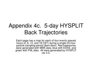
Objectives • Investigate ozone transport into Texas • Which source regions contribute to high ozone in Texas? • What effect do emissions changes in those source regions have on Texas ozone? • Use a suite of independent tools to analyze ozone transport • HYSPLIT back trajectories • Show pathways for air arriving at Texas monitors on high ozone days • New MM5CAMx-to-ARL tool reformats CAMx winds for input to HYSPLIT and calculates vertical velocities using CAMx algorithm • CAMx probing tools • APCA (Anthropogenic Precursor Culpability Assessment) • HDDM (Higher order Decoupled Direct Method)
Using APCA and HDDM to Study Modeled Transport • CAMx APCA and HDDM probing tools provide complementary information for transport analysis • APCA • Can quantify contributions by source region and source category to ozone at a given receptor and time • Does not give information about how such a contribution may change if emissions change • HDDM • Can provide estimates of model response to changes in emissions
APCA/HDDM Source Region Maps • APCA emissions source regions shown in red • HDDM emissions source regions shaded • Ohio and Tennessee Valleys (blue) • Southeastern U.S. (pink) • 3 emissions source categories • Elevated anthropogenic emissions • Biogenic emissions • All other emissions • Buffer around Texas, roughly corresponding to 12 km Texas domain
Episode Selection • Modeled three Texas high ozone episodes during 2005-6 • Episode selection based on monitoring network and model performance evaluation results • More rural ozone monitors in Texas during 2006 than 2005 • Focus on periods of high diagnosed and modeled transport from Ohio and Tennessee Valleys and Southeastern U.S. • June 13-15, 2006 • Good model performance in both 12 km grid and in source regions in 36 km grid; transport from OH-TN Valleys and SE diagnosed using HYSPLIT back trajectories
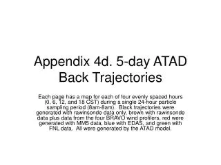
June 13-15, 2006 Transport Episode June 13 June 14 June 15 • Back trajectories from TCEQ analysis using EDAS meteorological inputs to HYSPLIT • Transport from OH-TN Valleys and SE into Texas
June 9-15, 2006: MPE for Source Regions • Good model performance with small positive bias Ohio/Tennessee Valleys Southeast Transport
Monitors Used in APCA/HDDM Analysis • Used rural monitors sited upwind of non-attainment areas • Selected monitors based on location and MPE • During transport episodes, evaluated source contributions with APCA at these receptors at the time of daily max 8-hour average ozone (DM8)
San Augustine, TX: June 14, 2006 • Largest contributions from Louisiana, Tennessee, BCs, other states in OH-TN Valley source region • APCA and HYSPLIT back trajectories are consistent in assessment of source regions
Ozone Sensitivity to Change in Elevated Anthro NOx Emissions in the Source Regions • Sensitivity of DM8 to elevated anthropogenic NOx (eaNOx) emissions in the OH-TN and SE source regions when > 60 ppb • For eaNOx only, calculate sensitivities S1OH-TN~∂O3 _____, S1SE ~ ∂O3_____, ∂(eaNOxOH-TN) ∂(eaNOxSE) S2 OH-TN~ ∂2O3________, S2SE ~ ∂2O3____, ∂(eaNOxOH-TN)2 ∂(eaNOxSE)2 where OT=Ohio and Tennessee Valleys, SE=Southeastern U.S. • How sensitive is East Texas ozone to emissions in these source regions?
June 13-15, 2006: Average S1OTand S2OT • S1OT generally positive and largest in source regions • Emissions increase generally would increase ozone; emissions reduction would decrease ozone • S1OT negative near large NOx sources; i.e. NOx reduction increases ozone (NOx disbenefit) • East-west S1OT gradient across Texas, 1-4 ppb on average over episode in East TX • S2OT largest in vicinity of large coal-fired power plants along the Ohio River
Sensitivity of Texas Ozone to Reductions in Source Region eaNOx • For a given monitor, calculate ozone change from emissions perturbation Δε using Taylor series expansion about unperturbed state, C(0) • C=ozone concentration, S(i) are sensitivities • Where Δε=-0.20 for 20% emissions reduction in the source region, for example, and C(0)=DM8 at the monitor in the unperturbed case • Neglecting higher order terms Rn+1 • Plot emissions change Δε versus change in ozone C(Δε)-C(0) at the monitor (next slide)
Change in Texas Ozone from Emissions Reduction in OH-TN Valley Source Region • Shows change in DM8 at rural TX monitors that would result from reducing eaNOx in OH-TN source region • NEWT and SAGA show largest ozone reductions
Zero-Out Contribution • HDDM coefficients can be used to estimate effect on ozone of removing (zeroing out) one or more emissions sources • For 2 emitters j and k, zero out contribution (ZOC) is calculated • For the OH-TN and SE source regions, ZOC is given by • ZOC(OT+SE)=(S(1)OT-½S(2)OT,OT)+ (S(1)SE-½S(2)SE,SE)- S(2)OT,SE • Here, we calculate components of ZOC for OH-TN and SE eaNOx emissions and present them separately, as cross term was negligible
Comparison of APCA and HDDM ZOC Estimates for eaNOx • The APCA and HDDM tools agree on the relative importance of these two source regions in contributing to high ozone in Texas • APCA and HDDM consistent with the HYSPLIT back trajectories APCA/HDDM HYSPLIT Back Trajectories
Conclusions • HYSPLIT, APCA and HDDM provide complementary information on • model winds that define transport pathways from source regions to receptor regions • ozone source apportionment • sensitivity of receptors to emissions changes in the source regions • Because their formulations are independent of one another, each of these tools can serve as a way to evaluate information provided by the others • Used in combination, these tools can provide a valuable resource for control strategy development.