Nyquist Plot

1. Nyquist Plot

2. What is a Nyquist Plot? Nyquist plot is a plot used mostly in control and signal processing and can be used to predict the stability and performance of a closed-loop system.

3. Nyquist Plot Nyquist plot is a plot of magnitude, and phase angle for frequency on s-plane.  (rad.s-1)  0 However we can obtain the sketch of the plot by obtaining the following vectors: • at (ii) at (iii) at , crossing on the real axis (iv) at , crossing on the imaginary axis

4. 1. Change Transfer Function From “s” Domain To “jw” Domain • First, If the transfer function G(s) is given in “s” domain, transfer it to “jω” domain. • Example: • Change it to:

5. 2. Find The Magnitude & Phase Angle Equations • Write an equation explaining the Magnitude and Phase Angle of the transfer function (now in “jω” form) that would look like: • For example the transfer function given above can be represented in the following form:

6. Note 1: The ω (Omega) value of “0+” means an angle very close to zero but slightly larger. The ε (epsilon) in the phase angle is due to ω being slightly larger than zero. This will be later used in drawing the nyquist plot. • Note 2: In above example, evaluating the phase angle (ω), at “0+” yields a phase angle of “-180 – ε”. The reason is that a slightly greater angle than zero would produce slightly greater “tangent” than zero.

7. 4. Find The Positions of “0+” & “+∞” On The Plot, And Connect Them • Using the values found from the above section, find the positions of “0+” and “+∞” on the Real and Imaginary axis: In the above example, the point at “0+” is located at “-180 - ε” degrees which is slightly more negative than “-180″. • Connect the points together. The second point is at “0″ on real axis with “-90″ degrees. Therefore the nyquist path coming from the “ω=0+” should approach the “ω=+∞” at a “-90″ degrees. The curvy path is not exact as we are only drawing the plot by hand. • Mirror the nyquist path plotted in part 2 across the real axis. • Connect the “ω=0-” to “ω=0+”. This should be done clock-wise. While in this example’s case the clock-wise path is the closest, that is not the case all the time.

8. Nyquist Plot Example • Consider the following transfer function: • Change it from “s” domain to “jω” domain: • Find the magnitude and phase angle equations:

9. Evaluate magnitude and phase angle at ω= 0+ and ω = +∞

10. Draw the nyquist plot: Pay attention that connecting the “0-” to “0+” point should be done in a clock-wise motion.

11. Example For the unity feedback system of Figure 1 below, where , sketch Nyquist diagram & evaluate its stability. Given K=1.

16. High Frequency Asymptotes   • How a Nyquist plot is affected when the system has a higher order?First, consider a more general transfer function.  Most transfer functions are a ratio of polynomials in s.  Here is a typical example - shown in factored form. • This system has m zeroes and n poles. • It is almost always true that the denominator is of higher order than the numerator so, • n  > m, i.e. #Poles > # Zeroes Although, on occasion we have: • n = m, i.e. #Poles = # Zeroes • The system has n poles and m zeroes. • Note that a stable system will have all of the poles in the left half of the s-plane, so all of the p's will be negative in G(s).  Also, zeroes will usually be in the left half of the s-plane, but it's possible that is not the case.

17. Now, let us assume - at least for the moment - that: The transfer function has no poles at s = 0 or the system has no poles at the origin. • We are going to examine the behavior of the Nyquist plot for large frequencies. • Let s = jω in the transfer function to obtain: Then, if we let the frequency become very large.  In the limit, each j ω term will "overpower" the corresponding z or p term in G(j ω) and we will have: G(j ω) ≈ 1/(j ω n-m) • The angle of this limiting form is determined by the j-term. • The angle is determined by the power of j.  You get -90o for every j. • For example, if n = 4, and m = 1, then n - m = 3, and for high frequencies the Nyquist plot would have an angle of -270o

18. A first order system, G(s) = 1/(s + 1) • The high frequency asymptote is at -90o which is where it should be for a system with one more pole than zero.

19. A second order system, G(s) = 1/(s + 1)2 • The high frequency asymptote is at -180o which is where it should be for a system with two more poles than zeroes.

20. A third order system, G(s) = 1/(s + 1)3 • The high frequency asymptote is at -270o which is where it should be for a system with three more poles than zeroes.

21. Here's a system with 5 poles and 2 zeroes. • Some poles are repeated - double - poles. • The complete Nyquist plot is below. • While the plot is fairly complex - especially for a system without any complex poles, the high frequency asymptote is still -270o.

22. Systems with complex poles can have resonant peaks.  Here is the transfer function of a system with complex poles. • Here is the Nyquist plot for the system.

23. The resonant peak causes the magnitude of the response to be larger than the DC gain (which is 1.0).  In the plot the DC gain is 1.0, and the plot starts from 1.  As the frequency increases the magnitude gets larger as the angle becomes negative.  It's a little larger than 1.6 when the phase reaches -90o. • It's also interesting to look at the density of points on the plot.  For these plots we have been using a logarithmic frequency spacing.  Looking at just the points, with no connecting lines between points, the plot below shows what you get.  In this plot we made the points a little larger (and messier, apparently!) than in the previous plots.  The negative frequency portion remains the same for comparison.

25. First order Frequency response Magnitude dan Phase angle

26. , , and (i) At , , dan (ii) At . i.e. or (iii) No crossing in the real axis as , (iv) No crossing in the imaginary axis as , is a circle.

27. Nyquist plot of Example: Frequency response , , and . At and At and >> nyquist([5],[.25 1])

29. Second Order Frequency response Rearrange

30. Magnitude Phase angle (i) at , and (ii) At , and . (iii) No crossing on the real axis. (iv) Crossing of the imaginary axis when , . and

31. Example: Frequency response Magnitude Phase angle

32. (i) At , (ii) At , and , (iii) Real axis crossing at , dan rad.s-1 or , Magnitude (iv) Imaginary crossing at , =0.6 rad.s-1 Magnitude »dr1=[2 1]; » dr2=[1 1 1]; » dr=conv(dr1,dr2); » nr=1; » nyquist(nr,dr)

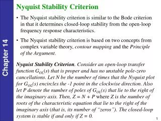
34. Nyquist Stability Criteria s-plane j For Nyquist path r  by replacing Contour of which will give the closed loop poles for till to become j satah-F(j) 

35. However Hence on F(j)-plane, we represent GH(j)-plane to plot j satah-GH(j) -1+j0  . where Z = Number of zeros on the right-half plane of j-axis. N = Numberof clockwise encirclement of P = Number of zeros on the right-half plane of j-axis.

36. Gain margin and Phase margin in Nyquist Plot satah-GH(j) j 1/GM  -1+j0

37. Is the measure of instability from on the -plane Phase crossover frequency, Frequency where the phase angle of is –180 o Gain crossover frequency, Frequency where the magnitude of Gain margin,

38. Example: For , shows the Nyquist plot and its respective gain and phase margin + - Open loop transfer function Frequency response

39. Magnitude Phase angle (i) At, and (ii) At, and

40. (iii) Real crossing, when . then Imaginary crossing, when (iv) then » nr=40; » dr1=[ 1 3]; » dr2=[1 4 7]; » dr=conv(dr1,dr2); » nyquist(nr,dr)

43. ADDITIONAL NOTES

44. Derivation of Nyquist Criterion

45. We conclude that, (1) the poles of 1+G(s)H(s) are the same as the poles of G(s)H(s) (2)the zeros of 1+G(s)H(s) are the same as the poles of T(s), the closed loop system. • The concept of mapping contour: • Consider a collection of points , called contour A can be mapped through a function F(s) into contour B by substituting each point of contour A into F(s).

46. The mapping of each point is defined by complex arithmetic, where the resulting complex number R is evaluated from the complex number represented by V.

48. If F(s) has just zeros or has just poles that are not encircled by the contour, mapping the points on contour A in a clockwise direction will map contour B in a clockwise direction. • Contour B maps in a counterclockwise direction if F(s) has just poles that are encircled by the contour A. • If the pole or zero of F(s) is enclosed by contour A, the mapping encircles the origin. • In the last case of Figure above, the pole and zero rotation cancel, the mapping does not encircle the origin.

49. As we move contour A in a clockwise direction, each vector that lies inside contour A will appear to undergo a complete rotation of 360o change in angle. • Each vector drawn from the poles and zeros that exist outside contour A will appear to oscillate and return to its position, undergoing a net angular change of 0o . • Moving in clockwise direction along the contour A, each zero inside contour A yields a rotation in the clockwise direction while each pole inside the contour A yields a rotation in an counterclockwise direction. • N=P-Z, • N equals the number of counterclockwise rotation of contour B. • P=number of poles of 1+G(s)H(s) inside contour A (number of enclosed open-loop pole) • Z=number of zeros of 1+G(s)H(s) inside contour A (number of enclosed close-loop poles)

50. Since all the poles and zero of G(s)H(s) are known, what if we map through G(s)H(s) instead of 1+G(s)H(s)? • The resulting contour is the same except that it is translated 1 unit to the left. We count rotation about -1 instead of rotation about the origin. • Nyquist Stability Criterion: If a contour A, that encircles the entire right half-plane is mapped through G(s)H(s), then the number of closed-loop poles, Z , in the right half plane equals the number of open loop poles, P, that are in the right half plane minus the number of the counterclockwise revolutions, N, around -1 of the mapping.