Stability from Nyquist plot
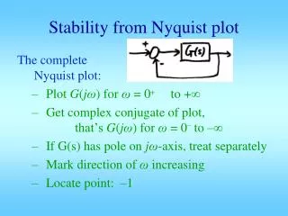
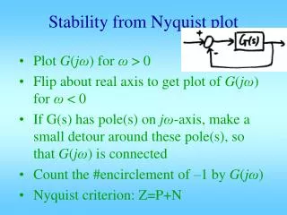
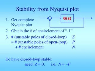
Stability from Nyquist plot. G(s). Get complete Nyquist plot Obtain the # of encirclement of “-1” # (unstable poles of closed-loop) Z = # (unstable poles of open-loop) P + # encirclement N To have closed-loop stable: need Z = 0, i.e. N = – P.

Stability from Nyquist plot
E N D
Presentation Transcript
Stability from Nyquist plot G(s) • Get completeNyquist plot • Obtain the # of encirclement of “-1” • # (unstable poles of closed-loop) Z= # (unstable poles of open-loop) P + # encirclement N To have closed-loop stable: need Z = 0, i.e. N = –P
Here we are counting only poles with positive real part as “unstable poles” • jw-axis poles are excluded • Completing the NP when there are jw-axis poles in the open-loop TF G(s): • If jwo is a non-repeated pole, NP sweeps 180 degrees in clock-wise direction as w goes from wo- to wo+. • If jwo is a double pole, NP sweeps 360 degrees in clock-wise direction as w goes from wo- to wo+.
Margins on Bode plots In most cases, stability of this closed-loop can be determined from the Bode plot of G: • Phase margin > 0 • Gain margin > 0 G(s)
Margins on Nyquist plot Suppose: • Draw Nyquist plot G(jω) & unit circle • They intersect at point A • Nyquist plot cross neg. real axis at –k
System type, steady state tracking C(s) Gp(s)
Type 0: magnitude plot becomes flat as w 0 phase plot becomes 0 deg as w 0 Kv = 0, Ka = 0 Kp = flat magnitude height near w 0
Asymptotic straight line Type 1: magnitude plot becomes -20 dB/dec as w 0 phase plot becomes -90 deg as w 0 Kp = ∞, Ka = 0 Kv = height of asymptotic line at w = 1 = w at which asymptotic line crosses 0 dB horizontal line
Asymptotic straight line Ka Sqrt(Ka) Type 2: magnitude plot becomes -40 dB/dec as w 0 phase plot becomes -180 deg as w 0 Kp = ∞, Kv = ∞ Ka = height of asymptotic line at w = 1 = w2at which asymptotic line crosses 0 dB horizontal line
Prototype 2nd order system frequency response For small zeta, resonance freq is about wn BW ranges from 0.5wn to 1.5wn For good z range, BW is 0.8 to 1.1 wn So take BW = wn z=0.1 0.2 0.3 No resonance for z <= 0.7 Mr=1dB for z=0.6 Mr=3dB for z=0.5 Mr=7dB for z=0.4
0.2 z=0.1 0.3 0.4 wgc In the range of good zeta, wgc is about 0.65 times to 0.8 times wn w/wn
In the range of good zeta, PM is about 100*z z=0.1 0.2 0.3 0.4 w/wn
Important relationships • Prototype wn, open-loop wgc, closed-loop BW are all very close to each other • When there is visible resonance peak, it is located near or just below wn, • This happens when z <= 0.6 • When z >= 0.7, no resonance • z determines phase margin and Mp: z 0.4 0.5 0.6 0.7 PM 44 53 61 67 deg ≈100z Mp 25 16 10 5 %
Important relationships • wgc determines wn and bandwidth • As wgc ↑, ts, td, tr, tp, etc ↓ • Low frequency gain determines steady state tracking: • L.F. magnitude plot slope/(-20dB/dec) = type • L.F. asymptotic line evaluated at w = 1: the value gives Kp, Kv, or Ka, depending on type • High frequency gain determines noise immunity