Download

1 / 31
310 likes | 443 Views
Geant 4 simulation of the DEPFET beam test. Daniel Scheirich, Peter Kodyš , Zdeněk Doležal, Pavel Řezníček Faculty of Mathematics and Physics Charles University, Prague. 2-12-2005, Prague. 2. Index. Geant 4 simulation program Model validation Geometry of the beam test

E N D
Geant 4 simulation of the DEPFET beam test Daniel Scheirich, Peter Kodyš, Zdeněk Doležal, Pavel Řezníček Faculty of Mathematics and Physics Charles University, Prague 2-12-2005, Prague
2 Index • Geant 4 simulation program • Model validation • Geometry of the beam test • Unscattered particles • Electron beam simulation • Residual plots for 2 different geometries • Residual plots for 3 different window thickness • CERN 180 GeV pion beam simulation • Conclusions
3 class TDetector class TDetector class TGeometry class TDetector class TGeometry … … Geant 4 simulation program • More about Geant 4 framework at www.cern.ch/geant4 • C++ object oriented architecture • Parameters are loaded from files G4 simulation program g4run.mac class TPrimaryGeneratorAction g4run.config class TDetectorConstruction detGeo1.config detGeo2.config … geometry.config det. position, det. geometry files sensitive wafers
4 Model validation • Simulation of an electron scattering in the 300m silicon wafer • Angular distribution histogram • Comparison with a theoretical shape of the distribution. According to the Particle Physics Review it is approximately Gaussian with a width given by the formula: where p, and z are the momentum, velocity and charge number, and x/X0 is the thickness in radiation length. Accuracy of 0 is 11% or better.
5 Example of an electron scattering Angular distribution electrons Silicon wafer
6 Gaussian fit Theoretical shape Non-gaussian tails
7 Results: simulation vs. theory 0… width of the theoretical Gaussian distribution …width of the fitted Gaussian accuracy of 0parametrisation (theory)is 11% or better Good agreement between the G4 simulation and the theory
8 Geometry of the beam test (DEPFET) Electron beam: 3x3 mm2, homogenous, parallel with x-axis
9 Geometry of the beam test: example
10 Configurations used for the simulation as planned for January 2006 TB – info from Lars Reuen, October 2005 Geometry 1 Module windows: • 50 m copper foils • no foils • 150 m copper foils Geometry 2 Module windows: • 50 m copper foils
11 Unscattered particle • Intersects of an unscattered particle lies on a straight line. • A resolution of telescopes is approximately pitch/(S/N) ~ 2 m. • Positions of intersects in telescopes plane were blurred with a Gaussian to simulate telescope resolution. • These points were fitted by a straight line.
12 Residual R(y) in DUT plane
14 =0.9912 m =0.9928 m =0.9918 m =0.9852 m
15 Unscattered particles: residual plots Geometry 1 = 1.19 m = 1.60 m = 1.60 m = 1.18 m = 0.99 m Geometry 2 = 1.05 m = 1.68 m = 1.68 m = 1.05 m = 0.99 m
16 Electron beamsimulation • There are 2 main contributions to the residual plots RMS: • Multiple scattering • Telescope resolution • Simulation was done for 1 GeV to 5 GeV electrons, 50000 events for each run • Particles that didn’t hit the both scintillators were excluded from the analysis • 2 cuts were applied to exclude bad fits
17 Example of 2 cuts 30% of events, 2 < 0.0005 50% of events, 2 < 0.0013 70% of events, 2 < 0.0025
18 Actual position DUT residual DUT plane Telescope resolution: Gaussian with =2 m
19 Electron beamsimulation: residual plots
20 Electron beamsimulation: residual plots
21 Residual-plot sigma vs. particle energy
22 Residual plots: two geometries Ideal detectors telescopes resolution included
23 Residual plots: two geometries Ideal detectors telescopes resolution included
24 Three windows thicknesses for the geometry 1 Geometry 1 • no foils • 50 m copper foils • 150 m copper foils Module windows:
25 Residual plots: three thicknesses Ideal detectors TEL & DUT resolution included
26 Residual plots: three thicknesses Ideal detectors TEL & DUT resolution included
27 Pion beam simulation • CERN 180 GeV pion beam was simulated • Geometries 1 and 2 were tested
28 Pion beam: residual plots Ideal detectors TEL & DUT resolution included
29 Pion beam: residual plots Ideal detectors TEL & DUT resolution included
30 Conclusions • Software for a simulation and data analysis has been created. Now it’s not a problem to run it all again with different parameters. • There is no significant difference between the geometry 1 and 2 for unscattered particles. • We can improve the resolution by excluding bad fits. • Geometry 2 gives wider residual plots due to amultiple scattering. For 5 GeV electrons and 30% 2 cut = 4.28 m for the Geometry 1 and = 5.94 m for the Geometry 2.
31 Conclusions • For 5 GeV electrons and 30% 2 cut there is approximately 1m difference between simulations with no module windows and 50 m copper windows. • CERN 180 GeV pion beam has a significantly lower multiple scattering. The main contribution to its residual plot width come from the telescopes intrinsic resolution.