Download
1 / 23
230 likes | 390 Views
Geant 4 simulation of the DEPFET beam test. Daniel Scheirich, Peter Kodyš , Zdeněk Doležal, Pavel Řezníček Faculty of Mathematics and Physics Charles University, Prague. 21-3-2006, Prague. 2. Content. Few words about program structure Model validation

E N D
Geant 4 simulation of the DEPFET beam test Daniel Scheirich, Peter Kodyš, Zdeněk Doležal, Pavel Řezníček Faculty of Mathematics and Physics Charles University, Prague 21-3-2006, Prague
2 Content • Few words about program structure • Model validation • Optimalization of the beam test geometry • Telescope resolutions • Comparison of simulation and measurement • Residual distributions • Infinite energy extrapolation • Confidence region of track • Prediction of DUT residual distribution width
Simulation program structure 3 class TDetector class TDetector class TGeometry class TDetector class TGeometry … … • More about Geant 4 framework at www.cern.ch/geant4 • C++ object oriented architecture • Parameters are loaded from files G4 simulation program g4run.mac class TPrimaryGeneratorAction g4run.config class TDetectorConstruction detGeo1.config detGeo2.config … geometry.config det. position, det. geometry files sensitive wafers
4 First step: model validation Gaussian fit Theoretical shape Simulation of an electron scattering in the 300m silicon wafer For this simple problem there is a good agreement between the G4 simulation and the theory
5 Geometry of the beam test • 4 telescopes in boxes with aluminium foil windows • DUT (DEPFET) in the middle • The whole set is enclosed by 2 scintillators used as a trigger Scintillator Telescopes DUT Scintillator
6 Residuals: telescopes & DUT Actual position TEL residual DUT residual DUT plane Telescope error Actual position In contrast to telescopes, DUT residual is a distance between the real position of intersect and the fitted one, hence we don’t know anything about DUT resolution
7 2 cuts … allow to exclude bad fits and improve residual distribution widths 30% of events, 2 < 0.0005 50% of events, 2 < 0.0013 70% of events, 2 < 0.0025
8 Before measurement: optimalization of the beam test geometry • Which geometry is better? • What is an influence of a window material thickness • How important is an influence of a multiple scattering and telescopes resolution? • What we gain if we use CERN 180 GeV pion beam instead of DESY electron beam? Few questions to be answered: OR Telescopes close together Far from each other
9 Results of geometry optimalization • Results of these simulations were presented in Bonn in December 2005 • Some plots and numbers: • There is no significant effect of 2 cuts Contribution of telescope intrinsic resolution: unscattered particles 2 cut : width 100% : =2.53 0.02m 70% : =2.53 0.02m 50% : =2.49 0.02 m 30% : =2.56 0.02m Telescope resolution 5 m
10 Results of geometry optimalization 2 cut Two geometries 100% 70% 50% 30% • Multiple scattering included • 2 cut does matter Geometry 1 is better
11 Results of geometry optimalization Window thickness • 0 m, 50 m and 150 m copper foils were tested in simulations • For 5 GeV electrons 50 m window makes 3 m difference in residual distribution compared to 0 m foil • After 30% 2 cut it makes only 1m • Multiple scattering is approx. 10 times lower than for electrons • The main contribution to residual distribution widths come from telescopes intrinsic resolution CERN 180 GeV pion beam
12 Final test beam geometry • Telescopes were placed as close as possible • 100 m aluminium foils were used as module windows 37 mm 34 mm 59 mm 37 mm
Telescopes intrinsic resolution 13 • Telescopes resolutions were set to values for that we get good correspondence between simulated and measured residual distributions • Analysis of measured data were made by Peter Kodyš • Telescopes points were fitted with straight line. All points had the same weight even though they were blurred with different Gaussian error distributions. Comparison of simulated residual distributions with measured ones @ 5 GeV Measurement Y side 7.8 6.5 [m] 7.2 6.1 Simulation 7.7 6.2 [m] 7.3 5.9 Measurement Z side 7.4 6.1 [m] 6.9 5.8 Simulation 7.5 6.0 [m] 7.1 5.8
Telescopes intrinsic resolution 14 • Telescopes resolutions were set to values for that we get good correspondence between simulated and measured residual distributions • Analysis of measured data were made by Peter Kodyš • Telescopes points were fitted with straight line. All points had the same weight even though they were blurred with different Gaussian error distributions. Comparison of simulated residual distributions with measured ones @ 5 GeV Measurement Obtained resolutions Y side 7.8 6.5 [m] 7.2 6.1 Simulation 7.7 6.2 [m] 7.3 5.9 Measurement Z side 7.4 6.1 [m] 6.9 5.8 Simulation 7.5 6.0 [m] 7.1 5.8
15 Simulation vs. measurement
16 Simulation vs. measurement
17 Simulation vs. measurement
18 Simulation vs. measurement
19 Infinite energy extrapolation Simulation Simulation Measurement 5.9 m 5.5 m Measurement 7.1 m 6.7 m Simulation Simulation Measurement 5.6 m 5.4 m Measurement 6.7 m 6.4 m
20 Confidence region of track Confidence region for estimation level 95% (2*sigma) was calculated in DUT position. Simulations: histogram of CRs Gaussian fit mean Sim. Mea. 6GeV 5GeV 4GeV 3GeV 2Gev 11.7 12.2 12.9 14.3 17.5 12 13 13 15 18 Confidence region DUT plane Example of CR histogram from measurement
21 Confidence region vs. residual distribution in DUT plane • From measurement: mean value of confidence region in DUT plane • From simulation: residual distribution in DUT plane & mean value of confidence region in DUT plane Measurement Simulation ?
22 Confidence region vs. residual distribution in DUT plane 1.08 1.28 1.45 1.58 1.71 CR/
23 Conclusions • Software for a simulation and data analysis has been created. I plan to implement magnetic field in the simulation. • Results of previous simulations were used for optimalization of beam test geometry. • A comparison of simulation and real data were made. Difference between residual distribution widths from simulation and measurement is lower than 1 m for energies 2 – 6 GeV. • A comparison was used to estimate mean value of telescopes intrinsic resolution. It fluctuate around 8m. • Regions of confidence (95%) in DUT plane were calculated from simulation and it was compared with ones from measurement. The numbers match very well. • Comparison of mean value of confidence region with residual distribution width in DUT plane was made. Ratio is an energy dependent.