Download
1 / 51
981 likes | 1.8k Views
CHAPTER 2. Time Domain Representation of Linear Time Invariant (LTI). School of Computer and Communication Engineering, UniMAP Nordiana Binti Mohamad Saaid dianams@unimap.edu.my. EKT 230. 2.0 Time Domain Representation of Linear Time Invariant (LTI) System. 2.1 Introduction.

E N D
CHAPTER 2 Time Domain Representation of Linear Time Invariant (LTI). School of Computer and Communication Engineering, UniMAP NordianaBintiMohamadSaaid dianams@unimap.edu.my EKT 230
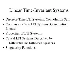
2.0 Time Domain Representation of Linear Time Invariant (LTI) System. 2.1 Introduction. 2.2 LTI System Properties. 2.3 Convolution Sum. 2.4 Convolution Integral. 2.5 Interconnection of LTI System. 2.6 LTI System Properties and Impulse Response. 2.7 The Step Response. 2.8 Solving Differential & Difference Equation.
Learning Outcome: Examine several methods for describing the relationship between the input and the output signals of LTI system. (1) Impulse Response. (2) Linear Constant-Coefficient Differential. (3) Block Diagram. 2.1 Introduction.
2.2 LTI System Properties. • If we know the response of the LTI system to some inputs, we actually know the response to many inputs. (1) Commutative Property.
Cont’d… (2) Distributive Property.
Cont’d… (3) Associative Property.
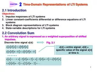
2.3 Convolution Sum. • x[n] is a signal as a weighted sum of basic function; time-shift version of the unit impulse signal. x[k] represents a specific value of the signal x[n] at time k. • The output of the LTI system y[n] is given by a weighted sum of time-shifted impulse response. h[n] is the impulse response of LTI system H. • The convolutionof two discrete-time signals y[n ] and h[n] is denoted as
Cont’d… Figure 2.1: Graphical example illustrating the representation of a signal x[n] as a weighted sum of time-shifted impulses.
Cont’d… Steps for Convolution Computation. Step 1:Plotx and h versus k since the convolution sum is on k. Step 2:Fliph[k] around the vertical axis to obtain h [- k]. Step 3:Shifth [-k] by n to obtain h [n- k]. Step 4:Multiply to obtain x[k] h[n- k]. Step 5:Sum on k to compute Step 6:Indexn and repeat Step 3-6.
Example 2.1:Convolution Sum. For the figure below, compute the convolution, y[n]. Figure 2.2a: Illustration of the convolution sum. (a) LTI system with impulse response h[n] and input x[n], producing y[n] and yet to be determined.
Solution: • Figure 2.2b: The decomposition of the input x[n] into a weighted sum of time shifted impulses results in an output y[n] given by a weighted sum of time-shifted impulse responses.
Example 2.2:Convolution. The LTI h[n] having an impulse response of and Solution: Details: Explained in class.
Example 2.3:Convolution. The LTI h[n] having an impulse response of and the input Find the convolution of, y[n]=x[n]*h[n]. Solution: • .
2.3.1 Convolution Sum Evaluation Procedure. • An alternative approach to evaluating the convolution sum. • Recall, the Convolution Sum is expressed as; define an intermediate signal as; so, • Time shift n determines the time at which we evaluated the output of the system. • The above formula is the simplified version of Convolution Sum, where we need to determine one signal wn[k] each time.
Example 2.4:Convolution Sum Evaluating by using an Intermediate Signal. Consider a system with impulse response Use the equation below to determine the output of the system at times n=-5, n =5, and n =10 when the input is x[n]=u[n]. Solution: In Figure 2.3 below x[k] is superimposed on the reflected and time-shifted impulse response h[n-k]. For n=-5, we have w-5[k]=0. This result in y[-5]=0. For n=5, we have The result is in Figure 2.3(c).
Cont’d… For n =10, we have The result is in Figure 2.3(d). Note: for n<0, wk[n]=0, because no overlap occur.
Cont’d… Figure 2.3: (a) The input signal x[k] above the reflected and time-shifted impulse response h[n – k], depicted as a function of k. (b) The product signal w5[k] used to evaluate y [–5]. (c) The product signal w5[k] used to evaluate y[5]. (d) The product signal w10[k] used to evaluate y[10].
2.4 Convolution Integral. • Derivation of Convolution Integral. (a) The operator H denotes the system in which the x(t) is applied. (b) Use the linearity property. (c) Define impulse response as unit impulse input.
Cont’d… • The time invariance implies that a time-shifted impulse input result in a time shift impulse response output as in Figure 2.4 below. Figure 2.4: (a) Impulse response of an LTI system H. (b) The output of an LTI system to a time-shifted and amplitude-scaled impulse is a time-shifted and amplitude-scaled impulse response.
Cont’d… To compute the superposition integral Step for Convolution Integral Computation. Step 1:Plotx and h versus t since the convolution sum is on t. Step 2:Fliph(t) around the vertical axis to obtain h(-t). Step 3:Shifth(t) by t to obtain h(t-t). Step 4:Multiply to obtain x(t) h(t-t). Step 5:Integrate on t to compute Step 6:Increaset and repeat Step 3-6.
t Example 2.5: Convolution Integral. Given a RC circuit below (RC=1s). Use convolution to determine the voltage across the capacitor y(t). Input voltage x(t)=u(t)-u(t-2). Solution: a y(t)=x(t)*h(t) - capacitor start charging at t=0 and discharging at t=2. b
Cont’d… • .
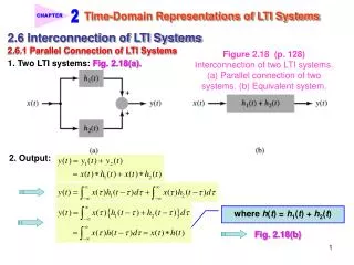
2.5 Interconnection of LTI System. • The objective of this section is to develop the relationship between the impulse response of an interconnection of LTI systems and impulse response of the constituent systems. 2.5.1 Parallel Connection of LTI System. 2.5.2 Cascade Connection of LTI System.
2.5.1 Parallel Connection of LTI Systems. • Two LTI systems with impulse response h1(t) and h2(t) connected in parallel, as in Figure 2.5 below. Figure 2.5: Interconnection of two LTI systems. (a) Parallel connection of two systems. (b) Equivalent system. • Derivation;
Cont’d… • Where h(t) = h1(t)+h2(t). • The impulse response of the overall system represented by the two LTI systems connected in parallel is the sum of their individual impulse response. • Distributive property of convolution (CT and DT),
2.5.2 Cascade Connection of Systems. • The impulse response an equivalent system representing two LTI systems connected in cascade is the convolution of their individual impulse responses. Figure 2.6: Interconnection of two LTI systems. (a) Cascade connection of two systems. (b) Equivalent system. (c) Equivalent system: Interchange system order.
Cont’d… • Derivation;
Cont’d… Continuous Time • Associative properties • Commutative properties. It is often used to simplify the evaluation or interpretation of the convolution integral. Discrete Time • Associative properties • Commutative properties.
Example 2.6: Equivalent System to Four Interconnected System. The interconnected of four LTI system is shown in figure below. Given the impulse response of the system, h1[n]=u[n] h2[n]=u[n+2]- u[n] h3[n]=d[n-2] and h4[n]=anu[n] h1[n]=u[n] Find the impulse response of the overall system. Solution: h[n]=(h1[n]+h2[n])*h3[n]-h4[n], Substitute the specific form of h1[n] and h2[n]to obtain. h12[n]=u[n]+u[n+2]-u[n] =u[n+2]
Cont’d… Convolving h12[n] with h3[n]. h123[n]= u[n]+u[n+2]*d[n] = u[n] Finally, we sum h123[n] and -h4[n] to obtain the overall impulse response: h[n]= {1-an}u[n]. Figure 2.7 : Interconnection of systems. • .
2.6 Relations between LTI System Properties and Impulse Response. • The impulse response characterized the input output behavior of an LTI system. Below are the propertiesof the system that relates to the impulse response. 2.6.1 Memoryless LTI Systems. 2.6.2 Causal LTI Systems. 2.6.3 Stable LTI Systems. 2.6.2 Invertible LTI Systems.
2.6.1 Memoryless LTI Systems. • The output of a memoryless system depends only on the present input. Continuous Time; Discrete Time;
2.6.2 Causal LTI Systems. • The output of a causal system depends only on the past input. Continuous Time; Discrete Time;
2.6.3 Stable LTI Systems. • Bounded Input Bounded Output (BIBO) stable system. • Discrete Time: absolute summability of the impulse response. • Continuous Time;
2.6.4 Invertible System and Deconvolution. • Deconvolution is the process of recovering x(t) from h(t)*x(t). • An exact inverse system may be difficult to find or implement. Determination of an approximate solution is often sufficient. • Figure 2.8: Cascade of LTI system with impulse response h(t) and inverse system with impulse response h-1(t).
2.7 Step Response. • Step response is defined as output due to a unit step input signal. • Step response s[t] of the discrete time is the running sum of the impulse response. • Step response s(t) of the continuous timesystem is the running integral of the impulse response. • Step response can be inverted to express in term of impulse response.
Example 2.7:RC Circuit of Step Response. The impulse response of the RC circuit is, Find the step response of the circuit. Solution: The step represented a switch that turns on a constant voltage source at time t=0. We expect the capacitor voltage to increase toward the value of the source in an exponential manner.
Cont’d… We simplify the integral to get Figure 2.9: RC circuit step response for RC = 1 s. • .
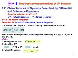
2.8 Solving Differential and Difference Equation. • The output of Differential and Difference Equation can be described as the sum of two components; (1) Homogeneous Solution y(h). (2) Particular Solution y(p). • The complete solution is y = y(h) +y(p) **Note: ( ) and [ ] are omit when referring to continuous and discrete time.
2.8.1 Homogeneous Solution. • Homogeneous form of difference and differential equation is obtained by setting all the terms involving the input to zero. Continuous-time System • Solution of homogeneous equation Equation (1) • Where the r1 are the N roots of the system’s characteristic equation • Substitution of equation (1) into the homogeneous equation results in y(h)(t) is a solution for any set of constant ci
Cont’d… Discrete-time System Solution of homogeneous equation Equation (2) Where the r1 are the N roots of the system’s characteristic equation Substitution of equation (2) into the homogeneous equation results in y(h)[t] is a solution for any set of constant ci. Note the CT and DT characteristic equations are different.
Example 2.9:Forced Response. The system is describe by the first order recursive system, Find the force response of the system if the input x[n]=(1/2)nu[n]. Solution: The difference between the previous example is the initial condition. Recall the complete solution is of the form To obtain c1, we translate the at-rest condition y[-1]=0 to time n=0 by noting that y[0]=1+(1/4)x0, now we know y[0]=1 and use to solve for c1. 1=2(1/2) 0 + c1(1/4)0 ; c1= -1 The force response is, • .
Block Diagram Representation. • Block diagram is an interconnection of elementary operations that act on the input signal. • A more detailed representation of the system than the impulse response or differential (difference) equation description since it describes how the system’s internal computations or operations are ordered. • Block diagram representations consists of an interconnection of three elementary operations on signals; (1) Scalar Multiplication. (2) Addition. (3) Integration for continuous-time LTI system.
Cont’d… Block Diagram Representation. Figure 2.10: Symbols for elementary operations in block diagram descriptions of systems. (a) Scalar multiplication. (b) Addition. (c) Integration for continuous-time systems and time shifting for discrete-time systems.
Example of Difference Equation: Discrete-Time System: Second Order Difference Equation. Figure 2.11: Block Diagram Representation of Discrete Time LTI system Described by second order Differential Equation.