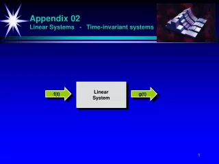
Linear Time Invariant systems

1. Linear Time Invariant systems • definitions, • Laplace transform, • solutions, • stability Lavi Shpigelman, Dynamic Systems and control – 76929 –

2. Lumpedness and causality • Definition: a system is lumped if it can be described by a state vector of finite dimension. Otherwise it is called distributed.Examples: • distributed system: y(t)=u(t- t) • lumped system (mass and spring with friction) • Definition:a system is causal if its current state is not a function of future events (all ‘real’ physical systems are causal) Lavi Shpigelman, Dynamic Systems and control – 76929 –

3. Linearity and Impulse Response description of linear systems • Definition: a function f(x) is linear if(this is known as the superposition property) Impulse response: • Suppose we have a SISO(Single Input Single Output) system system as follows: where: • y(t) is the system’s response (i.e. the observed output) to the control signal, u(t) . • The system is linear in x(t) (the system’s state) and in u(t) Lavi Shpigelman, Dynamic Systems and control – 76929 –

4. Linearity and Impulse Response description of linear systems • Define the system’s impulse response, g(t,), to be the response, y(t) of the system at time t, to a delta function control signal at time  (i.e. u(t)=t,t)given that the system state at time  is zero (i.e. x()=0 ) • Then the system response to anyu(t) can be found by solving: Thus, the impulse response contains all the information on the linear system Lavi Shpigelman, Dynamic Systems and control – 76929 –

5. causal relaxed Convolution Time invariant Time Invariance • A system is said to be time invariant if its response to an initial state x(t0) and a control signal u is independent of the value of t0. So g(t,) can be simply described as g(t)=g(t,0) • A linear time invariant system is said to be causal if • A system is said to be relaxed at time 0 if x(0)=0 • A linear, causal, time invariant (SISO) system that is relaxed at time 0can be described by Lavi Shpigelman, Dynamic Systems and control – 76929 –

6. Linear, 1st order ODEs Linear algebraic equations Dynamic Process ObservationProcess Controllable inputsu u D Observationsy B + x C 1/s + A State x Disturbance (noise) w Measurement Error (noise) n Plant LTI - State-Space Description Fact: (instead of using the impulse response representation..) • Every (lumped, noise free) linear, time invariant (LTI) system can be described by a set of equations of the form: Lavi Shpigelman, Dynamic Systems and control – 76929 –

7. What About nth Order Linear ODEs? • Can be transformed into n 1st order ODEs • Define new variable: • Then: Lavi Shpigelman, Dynamic Systems and control – 76929 – Dx/dt = A x + B u y = [I 0 0  0] x

8. Using Laplace Transform to Solve ODEs • The Laplace transform is a very useful tool in the solution of linear ODEs (i.e. LTI systems). • Definition: the Laplace transform of f(t) • It exists for any function that can be bounded byaet(and s>a) and it is unique • The inverse exists as well • Laplace transform pairsare known for many useful functions (in the form of tables and Matlab functions) • Will be useful in solving differential equations! Lavi Shpigelman, Dynamic Systems and control – 76929 –

9. Some Laplace Transform Properties • Linearity (superposition): • Differentiation Lavi Shpigelman, Dynamic Systems and control – 76929 –

10. Remember integration by parts: • Using that and the transform definition: Lavi Shpigelman, Dynamic Systems and control – 76929 –

11. Some Laplace Transform Properties • Linearity (superposition): • Differentiation • Convolution Lavi Shpigelman, Dynamic Systems and control – 76929 –

12. Using definitions • Integration over triangle 0 <  < t • Define  = t-t, thends = dt and region is  > 0, t> 0 Lavi Shpigelman, Dynamic Systems and control – 76929 –

13. Some Laplace Transform Properties • Linearity (superposition): • Differentiation • Convolution • Integration Lavi Shpigelman, Dynamic Systems and control – 76929 –

14. By definition: • Switch integration order • Plug  = t- Lavi Shpigelman, Dynamic Systems and control – 76929 –

15. Some specific Laplace Transforms (good to know) • Constant (or unit step) • Impulse • Exponential • Time scaling Lavi Shpigelman, Dynamic Systems and control – 76929 –

16. Homogenous (aka Autonomous / no input)1st order linear ODE • Solve: • Do the Laplace transform • Do simple algebra • Take inverse transform Lavi Shpigelman, Dynamic Systems and control – 76929 – Known as zero input response

17. 1st order linear ODE with input (non-homogenous) • Solve: • Do the Laplace transform • Do simple algebra • Take inverse transform Lavi Shpigelman, Dynamic Systems and control – 76929 – Known as the zero state response

18. Example: a 2nd order system • Solve: • Do the Laplace transform • Do simple algebra • Take inverse transform Lavi Shpigelman, Dynamic Systems and control – 76929 –

19. characteristic polynomial determined by Initial condition Using Laplace Transform to Analyze a 2nd Order system • Consider the autonomous (homogenous) 2nd order system • To find y(t), take the Laplace transform(to get an algebraic equation in s) • Do some algebra • Find y(t) by taking the inverse transform Lavi Shpigelman, Dynamic Systems and control – 76929 –

20. 2nd Order system - Inverse Laplace • Solution of inverse transform depends on nature of the roots1,2of the characteristic polynomial p(s)=as2+bs+c: • real & distinct, b2>4ac • real & equal, b2=4ac • complex conjugates b2<4ac • In shock absorber example:a=m, b=damping coeff.,c=spring coeff. • We will see: Re{} exponential effectIm{} Oscillatory effect Lavi Shpigelman, Dynamic Systems and control – 76929 –

21. p(s)=s2+3s+1y(0)=1,y’(0)=01=-2.622=-0.38 y(t)=-0.17e-2.62t+1.17e-0.38t Real & Distinct roots (b2>4ac) • Some algebra helps fit the polynomial to Laplace tables. • Use linearity, and a table entry To conclude: • Sign{}  growth or decay • ||  rate of growth/decay Lavi Shpigelman, Dynamic Systems and control – 76929 –

22. p(s)=s2+2s+1y(0)=1,y’(0)=01=-1 y(t)=-e-t+te-t Real & Equal roots (b2=4ac) • Some algebra helps fit the polynomial to Laplace tables. • Use linearity, and a some table entries to conclude: • Sign{}  growth or decay • ||  rate of growth/decay Lavi Shpigelman, Dynamic Systems and control – 76929 –

23. Complex conjugate roots (b2<4ac) • Some algebra helps fit the polynomial to Laplace tables. • Use table entries (as before) to conclude: • Reformulate y(t) in terms of  and Where: Lavi Shpigelman, Dynamic Systems and control – 76929 –

24. Complex conjugate roots (b2<4ac) • E.g. p(s)=s2+0.35s+1 and initial condition y(0)=1 , y’(0)=0 • Roots are =+i=-0.175±i0.9846 • Solution has form:with constantsA=||=1.0157r=0.5-i0.0889=arctan(Im(r)/Re(r)) =-0.17591 • Solution is an exponentially decaying oscillation • Decay governed by oscillation by . Lavi Shpigelman, Dynamic Systems and control – 76929 –

25. MarginallyStable Im(s) Stable Unstable Re(s) The “Roots” of a Response Lavi Shpigelman, Dynamic Systems and control – 76929 –

26. (Optional) Reading List • LTI systems: • Chen, 2.1-2.3 • Laplace: • http://www.cs.huji.ac.il/~control/handouts/laplace_Boyd.pdf • Also, Chen, 2.3 • 2nd order LTI system analysis: • http://www.cs.huji.ac.il/~control/handouts/2nd_order_Boyd.pdf • Linear algebra (matrix identities and eigenstuff) • Chen, chp. 3 • Stengel, 2.1,2.2 Lavi Shpigelman, Dynamic Systems and control – 76929 –