Download
1 / 69
830 likes | 1.54k Views
Chapter7 LTI Discrete-Time Systems in the Transform Domain. Transfer Function Classification Types of Linear-Phase Transfer Functions Simple Digital Filters. Types of Transfer Functions.

E N D
Chapter7 LTI Discrete-Time Systems in the Transform Domain Transfer Function Classification Types of Linear-Phase Transfer Functions Simple Digital Filters
Types of Transfer Functions • The time-domain classification of a digital transfer function based on the length of its impulse response sequence: - Finite impulse response (FIR) transfer function. - Infinite impulse response (IIR) transfer function.
Types of Transfer Functions • In the case of digital transfer functions with frequency-selective frequency responses, there are two types of classifications: (1) Classification based on the shape of the magnitude function |H(ei)|. (2) Classification based on the form of the phase function θ().
7.1 Transfer Function Classification Based on Magnitude Characteristics • Digital Filters with Ideal Magnitude Responses • Bounded Real Transfer Function • Allpass Transfer Function
7.1.1 Digital Filters with Ideal Magnitude Responses • A digital filter designed to pass signal components of certain frequencies without distortion should have a frequency response equal to 1 at these frequencies, and should have a frequency response equal to 0 at all other frequencies. • The range of frequencies where the frequency response takes the value of 1 is called the passband. • The range of frequencies where the frequency response takes the value of 0 is called the stopband.
Magnitude responses of the four popular types of ideal digital filters with real impulse response coefficients are shown below: • The frequencies c, c1, and c2are called the cutoff frequencies.
An ideal filter has a magnitude response equal to 1 in the passband and 0 in the stopband, and has a 0 phase everywhere. • The inverse DTFT of the frequency response HLP(ej) of the ideal lowpass filter is: hLP[n]=sincn/n, - <n< • We have shown that the above impulse response is not absolutely summable, and hence, the corresponding transfer function is not BIBO stable.
Also, hLP[n] is not causal and is of doubly infinite length. • The remaining three ideal filters are also characterized by doubly infinite, noncausal impulse responses and are not absolutely summable. • Thus, the ideal filters with the ideal “brick wall” frequency responses cannot be realizedwith finite dimensional LTI filter.
To develop stable and realizable transfer functions, the ideal frequency response specifications are relaxed by including a transition band between the passband and the stopband. • This permits the magnitude response to decay slowly from its maximum value in the passband to the 0 value in the stopband. • Moreover, the magnitude response is allowed to vary by a small amount both in the passband and the stopband.
Typical magnitude response specifications • of a lowpass filter are shown as:
Then the condition implies: for all values of w 7.1.2 Bounded Real Transfer Functions • A causal stable real-coefficient transfer function H(z) is defined as a bounded real (BR) transfer function if: • Let x[n] and y[n] denote, respectively, the input and output of a digital filter characterized by a BR transfer function H(z) with X(ejω) and Y(ejω) denoting their DTFTs.
Integrating the above from -π to π, and applying Parseval’s relation we get: • Thus, for all finite-energy inputs, the output energy is less than or equal to the input energy. • It implies that a digital filter characterized by a BR transfer function can be viewed as a passive structure.
A causal stable real-coefficient transfer function H(z) with is thus called a lossless bounded real (LBR) transfer function. If , then the output energy is equal to the input energy, and such a digital filter is therefore a lossless system. • The BR and LBR transfer functions are the keys to the realization of digital filters with low coefficient sensitivity.
Bounded Real Transfer Functions • Example: Consider the causal stable IIR transfer function: where K is a real constant. Its square-magnitude function is given by:
Thus, for α>0, ( |H(ejω)|2 )max = K2/(1- α)2 | ω=0 ( |H(ejω)|2 )min = K2/(1+α)2 | ω=π • On the other hand, for α<0, ( |H(ejω)|2 )max = K2/(1+α)2 | ω= π ( |H(ejω)|2 )min = K2/(1- α)2 | ω= 0 • Hence, is a BR function for K≤±(1-α).
Lowpass filter Highpass filter
Where a is real, and . Or a is complex, the H(z) should be: 7.1.3 Allpass Transfer Function • The magnitude response of allpass system satisfies: |A(ejω)|2=1, for all ω. • The H(z) of a simple 1th-order allpass system is:
An M-th order causal real-coefficient allpass transfer function is of the form: If we denote polynomial: Then:
We shall use the notation to denote the mirror-image polynomial of a degree-M polynomial DM(z) , i.e., • The numerator of a real-coefficient allpass transfer function is said to be the mirror-image polynomial of the denominator, and vice versa.
implies that the poles and zeros of a real-coefficient allpass function exhibit mirror-image symmetry in the z-plane. • The expression:
To show that |AM(ejω)|=1 we observe that: Therefore: Hence:
Figure below shows the principal value of the phase of the 3rd-order allpass function: • Note: The phase function of any arbitrary causal stable allpass function is a continuous function of ω.
Allpass Transfer Function • Properties: • A causal stable real-coefficient allpass transfer function is a lossless bounded real (LBR) function or, equivalently, a causal stable allpass filter is a lossless structure. • The magnitude function of a stable allpass function A(z) satisfies:
Let τg(ω) denote the group delay function of an allpass filter A(z), i.e., The unwrapped phase function θc(ω) of a stable allpass function is a monotonically decreasing function of w so that τg(ω) is everywhere positive in the range 0 < w < p.
G(z) A(z) Application of allpass system • Use allpass system to help design linear phase system---delay equalizer • Let G(z) be the transfer function of a digital filter designed to meet a prescribed magnitude response; • The nonlinear phase response of G(z) can be corrected by cascading it with an allpass filter A(z) so that the overall cascade has a constant group delay in the band of interest.
Since , we have • Overall group delay is the given by the sum of the group delays of G(z) and A(z). • Example: Figure below shows the group delay of a 4th order elliptic filter with the following specifications: ωp=0.3π, δp=1dB, δs=35dB
7.2 Transfer Function Classification Based on Phase Characteristic • Zero-Phase Transfer Function • Linear-Phase Transfer Function • Minimum-Phase and Maximum-Phase Transfer Functions
7.2.1 Zero-Phase Transfer Function • One way to avoid any phase distortions is to make the frequency response of the filter real and nonnegative,to design the filter with a zero phase characteristic. • However, it is impossible to design a causal digital filter with a zero phase.
v[n] w[n] u[n] x[n] H(z) H(z) u[n]=v[-n], y[n]=w[-n] • Only for non-real-time processing of real-valued input signals of finite length, the zero phase condition can be met. • One zero-phase filtering scheme is sketched below: • The function filtfilt implements the above zero-phase filtering scheme.
h[n] x[n] y[n] + Time- reversal h[n] Time- reversal • Another zero-phase filtering scheme is sketched in book P412—P7.5.
7.2.3 Minimum-Phase and Maximum-Phase Transfer Function • Consider the two 1st-order transfer functions: Both transfer functions have a pole inside the unit circle at the same location z=-a and are stable. • But the zero of H1(z) is inside the unit circle at z=-b, whereas, the zero of H2(z) is at z=1/b, situated in a mirror-image symmetry.
H1(z) H2(z) • Figure below shows the pole-zero plots of the two transfer functions: • Both transfer functions have an identical magnitude function.
The corresponding phase functions are: • Figure shows the unwrapped phase responses of the two transfer functions for a = 0.8 and b =-0.5
From this figure it follows that H2(z) has an excess phase lag with respect to H1(z). • The excess phase lag property of H2(z) with respect to H1(z) can also be explained by observing that: Where A(z) is a stable allpass function.
The phase functions of H1(z) and H2(z) are thus related through: arg[H2(ejω)]= arg[H1(ejω)]+ arg[A(ejω)] • As the unwrapped phase function of a stable first-order allpass function is a negative function of ω, it follows from the above that H2(z) has indeed an excess phase lag with respect to H1(z).
Generalizing the above result, letHm(z) be a causal stable transfer function with all zeros inside the unit circle and let H(z) be another causal stable transfer function satisfying |H(ejω)|= |Hm(ejω)|; • These two transfer functions are then related through H(z)=Hm(z)A(z) where A(z) is a causal stable allpass function. • The unwrapped phase functions of Hm(z) and H(z) are thus related through: arg[H(ejω)]= arg[Hm(ejω)]+ arg[A(ejω)] • H(z) has an excess phase lag with respect to Hm(z).
A causal stable transfer function with all zeros inside the unit circle is called a minimum-phase transfer function. • A causal stable transfer function with all zeros outside the unit circle is called a maximum-phase transfer function. • Any nonminimum-phase transfer function can be expressed as the product of a minimum-phase transfer function and a stable allpass transfer function. • A min-phase causal stable transfer function Hm(z) also has a delay that is smaller than the group delay of a nonmin-phase system which have the same magnitude response.
Example7.4: consider the mixed-phase transfer function: • We can rewrite H(z) as
7.2.2 Linear-Phase Transfer Function • The phase distortion can be avoided by ensuring that the transfer function has a unity magnitude and a linear-phase characteristic, that is: H(ejω)=e-jωD • Note: |H(ej)|=1, ()=D • The output y[n] of this filter to an input x[n]=Aejn is then given by: y[n]= Ae-jDejn =Aej(n-D)
If xa(t) and ya(t) represent the continuous-time signals whose sampled versions, sampled at t = nT, are x[n] and y[n] given above, then the delay between xa(t) and ya(t) is precisely the group delay of amount D. • If D is aninteger, then y[n] is identical to x[n], but delayed by D samples. • If D is not an integer, y[n], being delayed by a fractional part, is not identical to x[n].
If it is desired to pass input signal components in a certain frequency range undistorted in both magnitude and phase, then the transfer function should exhibit a unity magnitude response and a linear-phase response in the band of interest. • Since the signal components in the stopband are blocked, the phase response in the stopband can be of any shape.
Figure right shows the frequency response if a lowpass filter with a linear-phase characteristic in the passband
Example - Determine the impulse response of an ideal lowpass filter with a linear phase response: • Applying the frequency-shifting property of the DTFT to the impulse response of an ideal zero-phase lowpass filter we arrive at:
^ • By truncating the impulse response to a finite number of terms, a realizable FIR approximation to the ideal lowpass filter can be developed. • The truncated approximation may or may not exhibit linear phase, depending on the value of n0 chosen. • If we choose n0= N/2 with N a positive integer, the truncated and shifted approximation:
~ ^ ^ • Figure below shows the filter coefficients obtained using the function sinc for two different values of N.
7.3 Types of Linear-Phase FIR Transfer Functions • It is nearly impossible to design a linear-phase IIR transfer function. • It is always possible to design an FIR transfer function with an exact linear-phase response. • We now develop the forms of the linear-phase FIR transfer function H(z) with real impulse response h[n].
Where c and βare constants, and , called the amplitude function, also called the zero-phase response, is a real function of ω. 7.3.1 Linear-Phase FIR Transfer Functions • Consider a causal FIR transfer function H(z) of length N+1, i.e., of order N: • If H(z) is to have a linear-phase, its frequency response must be of the form:
Since , the amplitude response is then either an even or an odd function of ω, i.e., • For a real impulse response, the magnitude response |H(ejω)| is an even function of , i.e., |H(ejω)| = |H(e-jω)| • The frequency response satisfies the relation H(ejω)=H*(e-jω), or equivalently,
If is an even function, then the above relation leads to ejβ=e-jβ implying that either β=0 or β=π. Replacing ω with –ω in the equation we get: Therefore, we have
As , we have h[n]e-jω(c+n) = h[N-n]ejω(c+N-n) Making a change of variable l=N-n, we rewrite the equation as: The above leads to the condition: when c=-N/2,h[n]=h[N-n], 0≤n≤N