Linear Time-Invariant Systems
Linear Time-Invariant Systems. Quote of the Day The longer mathematics lives the more abstract – and therefore, possibly also the more practical – it becomes. Eric Temple Bell.

Linear Time-Invariant Systems
E N D
Presentation Transcript
Linear Time-Invariant Systems Quote of the Day The longer mathematics lives the more abstract – and therefore, possibly also the more practical – it becomes. Eric Temple Bell Content and Figures are from Discrete-Time Signal Processing, 2e by Oppenheim, Shafer, and Buck, ©1999-2000 Prentice Hall Inc.
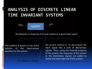
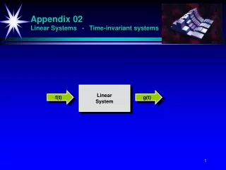
Linear-Time Invariant System • Special importance for their mathematical tractability • Most signal processing applications involve LTI systems • LTI system can be completely characterized by their impulse response • Represent any input • From time invariance we arrive at convolution [n-k] T{.} hk[n] 351M Digital Signal Processing
1 1 0.5 0.5 0 0 -5 0 5 -5 0 5 2 2 LTI LTI LTI LTI 1 1 0 0 -5 0 5 -5 0 5 2 2 1 1 0 0 -5 0 5 -5 0 5 2 4 1 2 0 0 -5 0 5 -5 0 5 LTI System Example 351M Digital Signal Processing
Convolution Demo Joy of Convolution Demo from John Hopkins University 351M Digital Signal Processing
x[n] h[n] y[n] h[n] x[n] y[n] h1[n] y[n] x[n] x[n] h1[n]+ h2[n] y[n] + h2[n] Properties of LTI Systems • Convolution is commutative • Convolution is distributive 351M Digital Signal Processing
Properties of LTI Systems • Cascade connection of LTI systems x[n] h1[n] h2[n] y[n] x[n] h2[n] h1[n] y[n] x[n] h1[n]h2[n] y[n] 351M Digital Signal Processing
Stable and Causal LTI Systems • An LTI system is (BIBO) stable if and only if • Impulse response is absolute summable • Let’s write the output of the system as • If the input is bounded • Then the output is bounded by • The output is bounded if the absolute sum is finite • An LTI system is causal if and only if 351M Digital Signal Processing
Linear Constant-Coefficient Difference Equations • An important class of LTI systems of the form • The output is not uniquely specified for a given input • The initial conditions are required • Linearity, time invariance, and causality depend on the initial conditions • If initial conditions are assumed to be zero system is linear, time invariant, and causal • Example • Moving Average • Difference Equation Representation 351M Digital Signal Processing
Eigenfunctions of LTI Systems • Complex exponentials are eigenfunctions of LTI systems: • Let’s see what happens if we feed x[n] into an LTI system: • The eigenvalue is called the frequency response of the system • H(ej) is a complex function of frequency • Specifies amplitude and phase change of the input eigenfunction eigenvalue 351M Digital Signal Processing
Eigenfunction Demo LTI System Demo From FernÜniversität, Hagen, Germany 351M Digital Signal Processing