Discrete-Time Signals: Time-Domain Representation

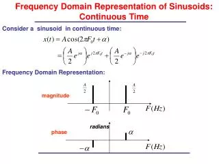
1. Discrete-Time Signals:Time-Domain Representation Tania Stathaki 811b t.stathaki@imperial.ac.uk

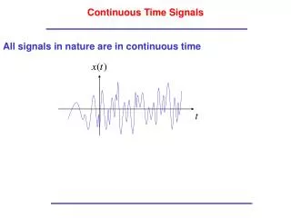
2. What is a signal ? A signal is a function of an independent variable such as time, distance, position, temperature, pressure, etc.

3. For example… • Electrical Engineering voltages/currents in a circuit speech signals image signals • Physics radiation • Mechanical Engineering vibration studies • Astronomy space photos

4. or • Biomedicine EEG, ECG, MRI, X-Rays, Ultrasounds • Seismology tectonic plate movement, earthquake prediction • Economics stock market data

6. What is DSP? Mathematical and algorithmic manipulation of discretized and quantized or naturally digital signals in order to extract the most relevant and pertinent information that is carried by the signal. What is a signal? What is a system? What is processing?

7. Signals can be characterized in several ways Continuous time signals vs. discrete time signals (x(t), x[n]). Temperature in London / signal on a CD-ROM. Continuous valued signals vs. discrete signals. Amount of current drawn by a device / average scores of TOEFL in a school over years. –Continuous time and continuous valued : Analog signal. –Continuous time and discrete valued: Quantized signal. –Discrete time and continuous valued: Sampled signal. –Discrete time and discrete values: Digital signal. Real valued signals vs. complex valued signals. Resident use electric power / industrial use reactive power. Scalar signals vs. vector valued (multi-channel) signals. Blood pressure signal / 128 channel EEG. Deterministic vs. random signal: Recorded audio / noise. One-dimensional vs. two dimensional vs. multidimensional signals. Speech / still image / video.

9. Systems • For our purposes, a DSP system is one that can mathematically manipulate (e.g., change, record, transmit, transform) digital signals. • Furthermore, we are not interested in processing analog signals either, even though most signals in nature are analog signals.

10. Various Types of Processing Modulation and demodulation. Signal security. Encryption and decryption. Multiplexing and de-multiplexing. Data compression. Signal de-noising. Filtering for noise reduction. Speaker/system identification. Signal enhancement –equalization. Audio processing. Image processing –image de-noising, enhancement, watermarking. Reconstruction. Data analysis and feature extraction. Frequency/spectral analysis.

11. Filtering • By far the most commonly used DSP operation Filtering refers to deliberately changing the frequency content of the signal, typically, by removing certain frequencies from the signals. For de-noising applications, the (frequency) filter removes those frequencies in the signal that correspond to noise. In various applications, filtering is used to focus to that part of the spectrum that is of interest, that is, the part that carries the information. • Typically we have the following types of filters Low-pass (LPF) –removes high frequencies, and retains (passes) low frequencies. High-pass (HPF) –removes low frequencies, and retains high frequencies. Band-pass (BPF) –retains an interval of frequencies within a band, removes others. Band-stop (BSF) –removes an interval of frequencies within a band, retains others. Notch filter –removes a specific frequency.

12. A Common Application: Filtering

13. Components of a DSP System

14. Components of a DSP System

15. Components of a DSP System

16. Analog-to-Digital-to-Analog…? • Why not just process the signals in continuous time domain? Isn’t it just a waste of time, money and resources to convert to digital and back to analog? • Why DSP? We digitally process the signals in discrete domain, because it is • 􀂪More flexible, more accurate, easier to mass produce. • 􀂪Easier to design. • System characteristics can easily be changed by programming. • Any level of accuracy can be obtained by use of appropriate number of bits. • 􀂪More deterministic and reproducible-less sensitive to component values, etc. • 􀂪Many things that cannot be done using analog processors can be done digitally. • Allows multiplexing, time sharing, multi-channel processing, adaptive filtering. • Easy to cascade, no loading effects, signals can be stored indefinitely w/o loss. • Allows processing of very low frequency signals, which requires unpractical component values in analog world.

17. Analog-to-Digital-to-Analog…? • On the other hand, it can be • 􀂪Slower, sampling issues. • 􀂪More expensive, increased system complexity, consumes more power. • Yet, the advantages far outweigh the disadvantages. Today, most continuous time signals are in fact processed in discrete time using digital signal processors.

18. Analog-Digital Examples of analog technology • photocopiers • telephones • audio tapes • televisions (intensity and color info per scan line) • VCRs (same as TV) Examples of digital technology • Digital computers!

19. In the next few slides you can see some real-life signals

20. Electroencephalogram (EEG) Data

21. Stock Market Data

22. Satellite imageVolcano Kamchatka Peninsula, Russia

23. Satellite imageVolcano in Alaska

24. Medical Images:MRI of normal brain

25. Medical Images:X-ray knee

26. Medical Images: UltrasoundFive-month Foetus (lungs, liver and bowel)

27. Astronomical images

28. Discrete-Time Signals:Time-Domain Representation • Signals represented as sequences of numbers, called samples • Sample value of a typical signal or sequence denoted asx[n]withnbeing an integer in the range • x[n] defined only for integer values of n and undefined for noninteger values ofn • Discrete-time signal represented by {x[n]}

29. Discrete-Time Signals:Time-Domain Representation • Here, n-th sample is given by • The spacing T is called the sampling interval or sampling period • Inverse of sampling interval T, denoted as , is called thesampling frequency:

30. Discrete-Time Signals:Time-Domain Representation • Two types of discrete-time signals: - Sampled-data signals in which samples are continuous-valued - Digital signals in which samples are discrete-valued • Signals in a practical digital signal processing system are digital signals obtained by quantizing the sample values either byroundingortruncation

31. 2 DimensionsFrom Continuous to Discrete: Sampling 256x256 64x64

32. Discrete (Sampled) and Digital (Quantized) Image

33. Discrete (Sampled) and Digital (Quantized) Image

34. Discrete (Sampled) and Digital (Quantized) Image 256x256 256 levels 256x256 32 levels

35. Discrete (Sampled) and Digital (Quantized) Image 256x256 256 levels 256x256 2 levels

36. Discrete-Time Signals:Time-Domain Representation • A discrete-time signal may be a finite-length or an infinite-length sequence • Finite-length (also called finite-duration or finite-extent) sequence is defined only for a finite time interval: where and with • Length or duration of the above finite-length sequence is

37. Discrete-Time Signals:Time-Domain Representation • A right-sided sequencex[n] has zero-valued samples for • If a right-sided sequence is called a causal sequence A right-sided sequence

38. Discrete-Time Signals:Time-Domain Representation • A left-sided sequencex[n] has zero-valued samples for • If a left-sided sequence is called a anti-causal sequence A left-sided sequence

39. Discrete-time system x[n] y[n] Output sequence Input sequence Operations on Sequences • A single-input, single-output discrete-time system operates on a sequence, called the input sequence, according some prescribed rules and develops another sequence, called the output sequence, with more desirable properties

40. Example of an Operation on a Sequence:Noise Removal • For example, the input may be a signal corrupted with additive noise • A discrete-time system may be designed to generate an output by removing the noise component from the input • In most cases, the operation defining a particular discrete-time system is composed of some basic operations

41. y[n] x[n] w[n] Basic Operations • Product (modulation) operation: • Modulator • An application is the generation of a finite-length sequence from an infinite-length sequence by multiplying the latter with a finite-length sequence called an window sequence • Process called windowing

42. y[n] x[n] w[n] A y[n] x[n] Basic Operations • Addition operation: • Adder • Multiplication operation • Multiplier

43. y[n] x[n] y[n] x[n] Basic Operations • Time-shifting operation: where N is an integer • If N > 0, it is a delay operation • Unit delay • If N < 0, it is an advance operation • Unit advance

44. x[n] x[n] x[n] Basic Operations • Time-reversal (folding) operation: • Branching operation: Used to provide multiple copies of a sequence

45. Combinations of Basic Operations • Example -

46. Sampling Rate Alteration • Employed to generate a new sequence y[n] with a sampling rate higher or lower than that of the sampling rate of a given sequencex[n] • Sampling rate alteration ratio is • If R > 1, the process called interpolation • If R < 1, the process called decimation

47. L Sampling Rate Alteration • In up-sampling by an integer factor L > 1, equidistant zero-valued samples are inserted by the up-sampler between each two consecutive samples of the input sequencex[n]:

48. Sampling Rate Alteration • An example of the up-sampling operation

49. M Sampling Rate Alteration • In down-sampling by an integer factor M > 1, every M-th samples of the input sequence are kept and in-between samples are removed:

50. Sampling Rate Alteration • An example of the down-sampling operation