Download
1 / 20
200 likes | 295 Views
Understand and apply the theorem for bivariate normal distribution with linear functions, constants, and correlation. Calculate probabilities, expectations, and more.

E N D
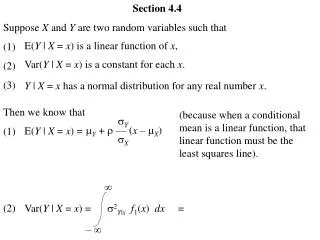
Section 4.4 Suppose X and Y are two random variables such that (1) (2) (3) E(Y | X = x) is a linear function of x, Var(Y | X = x) is a constant for each x. Y | X = x has a normal distribution for any real number x. Then we know that (1) (2) (because when a conditional mean is a linear function, that linear function must be the least squares line). Y Y+ — (x – X) X E(Y | X = x) = Var(Y | X = x) = 2Y|xf1(x)dx = –
Var(Y | X = x) = 2Y|xf1(x)dx = – 2 Y Y+ — (x – X) X y–h(y | x) dyf1(x)dx = – – 2 Y (y– Y) –— (x – X) X f(x,y) dydx = – – 2 Y (Y– Y) –— (X – X) = X E
2 Y (Y– Y) –— (X – X) = X E Y 2Y (Y– Y)2– 2— (X – X)(Y– Y) + 2— (X – X)2 = X 2X E Y 2Y E[(Y– Y)2] – 2— E[(X – X)(Y– Y)] + 2— E[(X – X)2] = X 2X Y 2 — Cov(X,Y) + X 2Y– 22Y = 2Y– 222Y+ 22Y = 2Y (1 – 2)
Suppose X and Y are two random variables such that (1) (2) (3) E(Y | X = x) is a linear function of x, Var(Y | X = x) is a constant for each x. Y | X = x has a normal distribution for any real number x, Then we know that (1) (2) Y Y+ — (x – X) X E(Y | X = x) = Var(Y | X = x) = 2Y (1 – 2) 2 Y – y– Y +— (x – X) X exp (3) For all x, h(y | x) = 22Y (1 – 2) – < y < (2)1/2Y (1 – 2)1/2
Now, suppose that X has a normal distribution. Then, the joint p.d.f. of (X,Y) is f(x,y) = f1(x) h(y | x) = 2 Y – y– Y +— (x – X) X exp – (x– X)2 exp 22X 22Y (1 – 2) = (2)1/2X (2)1/2Y (1 – 2)1/2 Y 2Y (y– Y)2– 2— (x – X)(y– Y) + 2— (x – X)2 X 2X 2 exp 1 x– X – — ——— – 2 X 22Y (1 – 2) = 2X Y (1 – 2)1/2
Y 2Y (y– Y)2– 2— (x – X)(y– Y) + 2— (x – X)2 X 2X 2 exp 1 x– X – — ——— – 2 X 22Y (1 – 2) = 2X Y (1 – 2)1/2 2 2 y– Yx – Xy– Yx – X ———– 2——— ——— + 2——— YX Y X 2 exp 1 x– X – — ——— – 2 X 2(1 – 2) = 2X Y (1 – 2)1/2
2 2 y– Yx – Xy– Yx – X ———– 2——— ——— + 2——— YX Y X 2 exp 1 x– X – — ——— – 2 X 2(1 – 2) = 2X Y (1 – 2)1/2 2 2 x – Xy– Yy – Y 2——— ——— + ——— X Y Y x– X ——— – X exp – < x < – < y < 2(1 – 2) 2X Y (1 – 2)1/2 (Note: Completing this derivation is Text Exercise 4.4-2.) This is called a bivariate normal p.d.f., and (X, Y) are said to have a bivariate normal distribution with correlation coefficient .
2 2 x – Xy– Yy – Y 2——— ——— + ——— X Y Y x– X ——— – X exp – < x < – < y < 2(1 – 2) 2X Y (1 – 2)1/2 From our derivation of the bivariate normal p.d.f., we know that (1) X has a N( X , 2X ) distribution, (2) Y | X = x has a N( , ) distribution. Y Y +— (x – X) X 2Y (1 – 2) From the symmetry of the bivariate normal p.d.f., we find that (1) Y has a distribution, (2) X | Y = y has a N( , ) distribution. N( Y , 2Y ) X X +— (y – Y) Y 2X (1 – 2)
Important Theorem in the Text: If (X, Y) have a bivariate normal distribution with correlation coefficient , then X and Y are independent if and only if = 0. Theorem 4.4-1
1. (a) Random variables X and Y are respectively the height (inches) and weight (lbs.) of adult males in a particular population. It is known that X and Y have a bivariate normal distribution with X = 70, Y = 150, X2 = 9, Y2 = 225, and = +0.4 . Find each of the following: P(140 < Y < 170) Y has a distribution. N( , ) 150 225 140 – 150 Y– 150 170 – 150 P( ———— < ——— < ———— ) = 15 15 15 P(140 < Y < 170) = P(– 0.67 < Z < 1.33) = (1.33)– (– 0.67) = (1.33)– (1 – (0.67)) = 0. 9082 – (1 – 0.7486) = 0.6568
1.-continued (b) P(X > 65) X has a distribution. N( , ) 70 9 X– 70 65 – 70 P( ——— > ———) = 3 3 P(X > 65) = P(Z > –1.67) = 1– (– 1.67) = 1– (1 – (1.67)) = 1 – (1 – 0.9525) = 0.9525
(c) (d) E(Y | X = x) Y Y+ — (x – X) = X 15 150 + 0.4— (x – 70) = 3 = 10 + 2x Var(Y | X = x) = 2Y (1 – 2) = 225(1 – 0.42) = 189
1.-continued (e) P(140 < Y < 170 | X = 72) Y | X = 72 has a distribution. N( , ) 154 189 140 – 154 Y– 154 170 – 154 P( ———— < ——— < ———— ) = 189 189 189 P(140 < Y < 170 | X = 72 ) = P(– 1.02 < Z < 1.16) = (1.16)– (– 1.02) = (1.16)– (1 – (1.02)) = 0. 8770 – (1 – 0.8461) = 0.7231
(f) P(140 < Y < 170 | X = 68) Y | X = 68 has a distribution. N( , ) 146 189 140 – 146 Y– 146 170 – 146 P( ———— < ——— < ———— ) = 189 189 189 P(140 < Y < 170 | X = 68 ) = P(– 0.44 < Z < 1.75) = (1.75)– (– 0.44) = (1.75)– (1 – (0.44)) = 0. 9599 – (1 – 0.6700) = 0.6299
1.-continued (g) P(140 < Y < 170 | X = 70) Y | X = 70 has a distribution. N( , ) 150 189 140 – 150 Y– 150 170 – 150 P( ———— < ——— < ———— ) = 189 189 189 P(140 < Y < 170 | X = 70 ) = P(– 0.73 < Z < 1.45) = (1.45)– (– 0.73) = (1.45)– (1 – (0.73)) = 0.9265 – (1 – 0.7673) = 0.6938
(h) (i) E(X | Y = y) X X+ — (y – Y) = Y 3 70 + 0.4— (y – 150) = 15 = 58 + 0.08y Var(X | Y = y) = 2X (1 – 2) = 9(1 – 0.42) = 7.56
1.-continued (j) P(X > 65 | Y = 140) X | Y = 140 has a distribution. N( , ) 69.2 7.56 X– 69.2 65 – 69.2 P( ———— > ———— ) = 7.567.56 P(X > 65 | Y = 140 ) = P(Z > – 1.53) = 1– (– 1.53) = 1– (1 – (1.53)) = 1 – (1 – 0.9370) = 0.9370
2. (a) (b) (c) (d) (e) (f) The random variables X and Y have a bivariate normal distribution with X = 10, Y = 5, X2 = 16, Y2 = 36, and = –0.4 . Find each of the following: Complete #2 for homework! 10 + 5 = 15 E(X + Y) = 16 + 36 + 2(–0.4)(16)1/2(36)1/2 = 32.8 Var(X + Y) = 10 – 5 = 5 E(X–Y) = 16 + 36 – 2(–0.4)(16)1/2(36)1/2 = 71.2 Var(X–Y) = 10 – 3(5) = – 5 E(X– 3Y) = Var(X– 3Y) = 16 + (–3)2(36) + (2)(–3)(–0.4)(16)1/2(36)1/2 = 397.6
3. (a) (b) Suppose the random variables X and Y have joint p.d.f. – (x2 + y2)/2 1 – (x2 + y2)/2 e + xy e – < x < if – < y < f(x,y) = 2 Are X and Y independent? Why or why not? Since f(x,y) cannot be factored into the product of a function of x alone and a function of y alone, then X and Y cannot possibly be independent. Find the marginal p.d.f. of X and the marginal p.d.f. of Y. – (x2 + y2)/2 1 – (x2 + y2)/2 e + xy e f1(x) = dy = 2 –
– (x2 + y2)/2 1 – (x2 + y2)/2 e xy e dy + dy 2 2 – – This is a bivariate normal p.d.f. with X = , 2X = , Y = , 2Y = , and = . This is an odd function, which implies that the integral of this function is . 0 1 0 1 0 Consequently, f1(x) is a N(0,1) p.d.f., and similarly we see that f2(y) is a N(0,1) p.d.f. 0 (c) Decide whether each of the following statements is true or false: True If (X, Y) have a bivariate normal distribution, then the marginal distribution for each of X and Y must be a normal distribution. False If the marginal distribution for each of X and Y is a normal distribution, then (X, Y) must have a bivariate normal distribution.