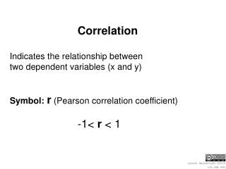
Section 10.2 Correlation between two variables ( x and y )
430 likes | 443 Views
Learn about the linear correlation coefficient, interpreting correlation, no correlation, and methods to determine if two variables are correlated using StatCrunch and critical regions or P-value analysis.

Section 10.2 Correlation between two variables ( x and y )
E N D
Presentation Transcript
Section 10.2Correlation between two variables (x and y) Objective Investigate how two variables (x and y) are related (i.e. correlated). That is, how much they depend on each other.
Definitions Acorrelationexists between two variables when the values of one appears to somehow affect the values of the other in some way. In this class, we are only interested in linear correlation
Definitions Linear correlation coefficient : r A numerical measure of the strength of the linear relationship between two variables, x and y, representing quantitative data. r always belongs in the interval (-1,1) ( i.e. –1 r 1 ) We use this value to conclude if there is(or is not) a linear correlation between the two variables.
Exploring the Data We can often see a relationship between two variables by constructing a scatterplot.
Positive Correlation We say the data has positive correlation if the data follows a line (with a positive slope). The correlation coefficient (r) will be close to +1
Negative Correlation We say the data has negative correlation if the data follows a line (with a negative slope). The correlation coefficient (r) will be close to –1
No Correlation We say the data has no correlation if the data does not seem to follow any line. The correlation coefficient (r) will be close to 0
Interpreting r r≈ 1Strong positive linear correlation r≈ 0Weak linear correlation r≈ -1 Strongnegative linear correlation
Nonlinear Correlation The data may follow a curve, but if the data is not linear, the linear correlation coefficient (r) will be close to zero.
1. The sample of paired (x, y) data is a random sample of quantitative data. 2. Visual examination of the scatterplot must confirm that the points approximate a straight-line pattern. 3. The outliers must be removed if they are known to be errors. (Note: We will not do this in this course) Requirements
n Number of pairs of sample data Denotes the addition of the items x The sum of all x-values x = x1 + x2 +…+ xn y The sum of all y-values y = y1 + y2 +…+ yn Notation
x2 The sum of the squares for all x-values x2=x12 + x22 +…+ xn2 (x)2The sum of the x-values, then squared (x)2=(x1 + x2 +…+ xn)2 xy The sum of the products of x and y xy=x1y1 + x1y2 +…+ xnyn Notation
rSamplelinear correlation coefficient r Populationlinear correlation coefficient (i.e. the linear correlation between the two populations) n(xy)–(x)(y) r= n(x2)– (x)2n(y2)– (y)2 Correlation Coefficient r measures the strength of a linear relationship between the paired values in a sample. We use StatCrunch compute r(Don’t panic!)
Example 1a Make a scatterplot for the heights of mother , daughter Enter data on StatCrunch(Mother in 1st column, daughter in 2nd column) 1
Example 1a Make a scatterplot for the heights of mother , daughter 2 Graphics – Scatter Plot
Example 1a Make a scatterplot for the heights of mother , daughter Select var1 for X variable (height of mother) Select var2 for Y variable (height of daughter) Click Create Graph! 3
Example 1a Make a scatterplot for the heights of mother , daughter 4 Voila! (Does there appear to be correlation?)
Example 1b Find the linear correlation coefficient of the heights 1 Stat – Summary Stats – Correlation
Example 1b Find the linear correlation coefficient of the heights Select var1 andvar2 so they appear in the right box Click Calculate 2
Example 1b Find the linear correlation coefficient of the heights 3 The Correlation Coefficient is r=0.802 (rounded)
Determining if Correlation Exists We determine whether a population is correlated via a two-tailed teston a sample using a significance level (α) H0 : ρ=0 (i.e. not correlated) H1 : ρ≠0 (i.e. is correlated) Again, two methods available: Critical Regions (Use TableA-6) P-value (Use StatCrunch) Note: In most cases we use significance level a = 0.05
Using Critical Regions Use Table A-6 to find the critical values, which depends on the sample size n. Use both positive a negative values (two-tailed) ● If the r is in the critical region, we conclude that there is a linear correlation. (Since H0 is rejected) ● If the r is not in the critical region, we say there is insufficient evidence of correlation. (Since we fail to rejectH0) -1 1 0
Example 1c Use a 0.05 significance level to determine if the heights are linearly correlated. UsingCritical Regions ● From Example 1b, we found r = 0.802 ● Since n = 20 and α = 0.05, using Table A-6, we find the critical values to be: 0.444, -0.444 Since r is in the critical region (reject H0), we conclude the data is linearly correlated (under 0.05 significance).
Using P-value Use StatCrunch to calculate the two-tailed P-value from a sample set (see Example 1c) ● If the P-value is less than α, we conclude that there is a linear correlation. (Since H0 is rejected) ● If the P-value is greater than α, we say there is insufficient evidence of correlation. (Since we fail to reject H0)
Example 1c Use a 0.05 significance level to determine if the heights are linearly correlated. UsingP-value ● On StatCrunch: Stat – Summary Stats – Correlation ● Select var1,var2 so they appear in right box Click Next ● Check “Display two-sides P-value from sig. test” ClickCalculate ● Result: P-value < 0.0001 Since P-value is less than α=0.05 (reject H0), we conclude the data is linearly correlated
Caution! Know that the methods of this section apply only to a linearcorrelation. If you conclude that there is no linear correlation, it is possible that there is some other association that is not linear.
Round r to three decimal places so that it can be compared to critical values in Table A-6 Rounding the Linear Correlation Coefficient
1.–1 r 1 2. If all values of either variable are converted to a different scale, the value of rdoes not change. 3. The value of r is not affected by the choice of x and y. Interchange all x-values and y-valuesand the value of rwill not change. 4.rmeasures strength of a linear relationship. 5.r is very sensitive to outliers, they can dramatically affect its value. Properties of the Linear Correlation Coefficient r
Example 2 A new medication for high blood pressure was tested on a batch of 18 patients with different ages. The results were as follows: (a) Plot the points (b) Find the correlation coefficient (c) Use a 0.05 significance level to test linear correlation
Example 2a Plot the points ● Enter data in StatCrunch ● Go to: Graphics – Scatter Plot ● Selectvar1andvar2, hitCreate Graph!
Example 2b Find Correlation Coefficient ● Go to: Stats – Summary Stats – Correlation ● Selectvar1andvar2, hitCalculate r = 0.964
Example 2c Test for Correlation (α= 0.05) Using Critical Values Given n=18 and α=0.05, using Table A-6, the critical values are 0.468, -0.468 r = 0.964 Since r is in the critical region, (reject H0), we conclude there islinear correlation
Example 2c Test for Correlation (α= 0.05) Using P-value ● Go to: Stats – Summary Stats – Correlation ● Selectvar1andvar2, hitNext ● Check box, hitCalculate r = 0.964 P-value < 0.0001 Since P-valueless thanα=0.05 (reject H0), we conclude there islinear correlation
Example 3 A survey of 15 people was conducted to see how many friends people had on Facebook vs. their shoe size. The results were as follows: (a) Plot the points (b) Find the correlation coefficient (c) Use a 0.05 significance level to test linear correlation
Example 3a Plot the points ● Enter data in StatCrunch ● Go to: Graphics – Scatter Plot ● Selectvar1andvar2, hitCreate Graph!
Example 3b Find Correlation Coefficient ● Go to: Stats – Summary Stats – Correlation ● Selectvar1andvar2, hitCalculate r = 0.409
Example 3c Test for Correlation (α= 0.05) Using Critical Values Given n=15 and α=0.05, using Table A-6, the critical values are 0.514, -0.514 r = 0.409 Since r is not in the critical region, (fail to reject H0), we conclude there is no correlation
Example 3c Test for Correlation (α= 0.05) Using P-value ● Go to: Stats – Summary Stats – Correlation ● Selectvar1andvar2, hitNext ● Check box, hitCalculate r = 0.409 P-value = 0.1297 Since P-valuegreater thanα=0.05 (fail to reject H0), we conclude there is no correlation
Interpreting r:Explained Variation The value of r2 is the proportion of the variation in y that is explained by the linear relationship between x and y. Low variance High variance r = 0.623 r 2 = 0.388 r = 0.998 r 2 = 0.996
Example 4 Using the data in Example 2 (blood pressure vs. age), we found that the linear correlation coefficient is r = 0.964 What proportion of the variation in the patients’ blood pressure can be explained by the variation in the patients’ age? With r = 0.964, we get r2 = 0.929 We conclude that 0.929 (or about 93%) of the variation in blood pressure can be explained by the linear relationship between the age and blood pressure. This implies about 7% of the variation in blood pressure cannot be explained by the age.
1. Causation: It is wrong to conclude that correlation implies causality. 2. Linearity: There may be some relationship between x and y even when there is no linear correlation. Common Errors Involving Correlation
Know that correlation does not implycausality. There may be correlation without causality. Caution!!!