Download
1 / 61
610 likes | 736 Views
Learn to determine binomial conditions, compute probabilities, calculate mean and SD in binomial setting, and probabilities involving geometric random variables. Explore examples and understand the concepts of binomial coefficients and probabilities.

E N D
Section 6.3Binomial and Geometric Random Variables Learning Objectives After this section, you should be able to… • DETERMINE whether the conditions for a binomial setting are met • COMPUTE and INTERPRET probabilities involving binomial random variables • CALCULATE the mean and standard deviation of a binomial random variable and INTERPRET these values in context • CALCULATE probabilities involving geometric random variables
Binomial Settings When the same chance process is repeated several times, we are often interested in whether a particular outcome does or doesn’t happen on each repetition. In some cases, the number of repeated trials is fixed in advance and we are interested in the number of times a particular event (called a “success”) occurs. If the trials in these cases are independent and each success has an equal chance of occurring, we have a binomial setting. Definition: A BINOMIAL SETTING arises when we perform several independent trials of the same chance process and record the number of times that a particular outcome occurs. The four conditions for a binomial setting are • Binary? The possible outcomes of each trial can be classified as “success” or “failure.” B • Independent? Trials must be independent; that is, knowing the result of one trial must not have any effect on the result of any other trial. I N • Number? The number of trials n of the chance process must be fixed in advance. S • Success? On each trial, the probability p of success must be the same.
Binomial Random Variable Consider tossing a coin n times. Each toss gives either heads or tails. Knowing the outcome of one toss does not change the probability of an outcome on any other toss. If we define heads as a success, then p is the probability of a head and is 0.5 on any toss. The number of heads in n tosses is a binomial random variable X. The probability distribution of X is called a binomial distribution. Definition: The count X of successes in a binomial setting is a binomial random variable. The probability distribution of X is a binomial distribution with parameters n and p, where n is the number of trials of the chance process and p is the probability of a success on any one trial. The possible values of X are the whole numbers from 0 to n. Note: When checking the Binomial condition, be sure to check the BINS and make sure you’re being asked to count the number of successes in a certain number of trials!
Binomial and Geometric Random Variables • Binomial Probabilities In a binomial setting, we can define a random variable (say, X) as the number ofsuccesses in n independent trials. We are interested in finding the probability distribution of X. Example Each child of a particular pair of parents has probability 0.25 of having type O blood. Genetics says that children receive genes from each of their parents independently. If these parents have 5 children, the count X of children with type O blood is a binomial random variable with n = 5 trials and probability p = 0.25 of a success on each trial. In this setting, a child with type O blood is a “success” (S) and a child with another blood type is a “failure” (F). What’s P(X = 2)? P(SSFFF) = (0.25)(0.25)(0.75)(0.75)(0.75) = (0.25)2(0.75)3 = 0.02637 However, there are a number of different arrangements in which 2 out of the 5 children have type O blood: SSFFF SFSFF SFFSF SFFFS FSSFF FSFSF FSFFS FFSSF FFSFS FFFSS Verify that in each arrangement, P(X = 2) = (0.25)2(0.75)3 = 0.02637 Therefore, P(X = 2) = 10(0.25)2(0.75)3 = 0.2637
Binomial and Geometric Random Variables • Binomial Coefficient Note, in the previous example, any one arrangement of 2 S’s and 3 F’s had the same probability. This is true because no matter what arrangement, we’d multiply together 0.25 twice and 0.75 three times. We can generalize this for any setting in which we are interested in k successes in n trials. That is,
Definition: The number of ways of arranging k successes among n observations is given by the binomial coefficient for k = 0, 1, 2, …, n where n! = n(n – 1)(n – 2)•…•(3)(2)(1) and 0! = 1.
Binomial and Geometric Random Variables • Binomial Probability The binomial coefficient counts the number of different ways in which k successes can be arranged among n trials. The binomial probability P(X = k) is this count multiplied by the probability of any one specific arrangement of the k successes. Binomial Probability If X has the binomial distribution with n trials and probability p of success on each trial, the possible values of X are 0, 1, 2, …, n. If k is any one of these values, Number of arrangements of k successes Probability of n-k failures Probability of k successes
Example: Inheriting Blood Type Each child of a particular pair of parents has probability 0.25 of having blood type O. Suppose the parents have 5 children (a) Find the probability that exactly 3 of the children have type O blood. Let X = the number of children with type O blood. We know X has a binomial distribution with n = 5and p = 0.25. (b) Should the parents be surprised if more than 3 of their children have type O blood? To answer this, we need to find P(X > 3). Since there is only a 1.5% chance that more than 3 children out of 5 would have Type O blood, the parents should be surprised!
Binomial and Geometric Random Variables • Mean and Standard Deviation of a Binomial Distribution We describe the probability distribution of a binomial random variable just like any other distribution – by looking at the shape, center, and spread. Consider the probability distribution of X = number of children with type O blood in a family with 5 children. Shape: The probability distribution of X is skewed to the right. It is more likely to have 0, 1, or 2 children with type O blood than a larger value. Center: The median number of children with type O blood is 1. Based on our formula for the mean: Spread: The variance of X is The standard deviation of X is
Binomial and Geometric Random Variables • Mean and Standard Deviation of a Binomial Distribution Notice, the mean µX= 1.25 can be found another way. Since each child has a 0.25 chance of inheriting type O blood, we’d expect one-fourth of the 5 children to have this blood type. That is, µX= 5(0.25) = 1.25. This method can be used to find the mean of any binomial random variable with parameters n and p. Mean and Standard Deviation of a Binomial Random Variable If a count X has the binomial distribution with number of trials n and probability of success p, the mean and standard deviation of X are Note: These formulas work ONLY for binomial distributions. They can’t be used for other distributions!
Example: Bottled Water versus Tap Water Mr. Bullard’s 21 AP Statistics students did the Activity on page 340. If we assume the students in his class cannot tell tap water from bottled water, then each has a 1/3 chance of correctly identifying the different type of water by guessing. Let X = the number of students who correctly identify the cup containing the different type of water. Find the mean and standard deviation of X. Since X is a binomial random variable with parameters n = 21 and p = 1/3, we can use the formulas for the mean and standard deviation of a binomial random variable. If the activity were repeated many times with groups of 21 students who were just guessing, the number of correct identifications would differ from 7 by an average of 2.16. We’d expect about one-third of his 21 students, about 7, to guess correctly.
Binomial and Geometric Random Variables • Binomial Distributions in Statistical Sampling The binomial distributions are important in statistics when we want to make inferences about the proportion p of successes in a population. Suppose 10% of CDs have defective copy-protection schemes that can harm computers. A music distributor inspects an SRS of 10 CDs from a shipment of 10,000. Let X = number of defective CDs. What is P(X = 0)? Note, this is not quite a binomial setting. Why? The actual probability is Using the binomial distribution, In practice, the binomial distribution gives a good approximation as long as we don’t sample more than 10% of the population. Sampling Without Replacement Condition When taking an SRS of size n from a population of size N, we can use a binomial distribution to model the count of successes in the sample as long as
Normal Approximation for Binomial Distributions As n gets larger, something interesting happens to the shape of a binomial distribution. The figures below show histograms of binomial distributions for different values of n and p. What do you notice as n gets larger?
Normal Approximation for Binomial Distributions Suppose that X has the binomial distribution with n trials and success probability p. When n is large, the distribution of X is approximately Normal with mean and standard deviation As a rule of thumb, we will use the Normal approximation when n is so large that np≥ 10 and n(1 – p) ≥ 10. That is, the expected number of successes and failures are both at least 10.
Example: Attitudes Toward Shopping Sample surveys show that fewer people enjoy shopping than in the past. A survey asked a nationwide random sample of 2500 adults if they agreed or disagreed that “I like buying new clothes, but shopping is often frustrating and time-consuming.” Suppose that exactly 60% of all adult US residents would say “Agree” if asked the same question. Let X = the number in the sample who agree. Estimate the probability that 1520 or more of the sample agree. 1) Verify that X is approximately a binomial random variable. B: Success = agree, Failure = don’t agree I: Because the population of U.S. adults is greater than 25,000, it is reasonable to assume the sampling without replacement condition is met. N: n = 2500 trials of the chance process S: The probability of selecting an adult who agrees is p = 0.60 2) Check the conditions for using a Normal approximation. Since np = 2500(0.60) = 1500 and n(1 – p) = 2500(0.40) = 1000 are both at least 10, we may use the Normal approximation.
The number X of switches that fail inspection has approximately the binomial distribution with n = 10 and p = 0.1. • What is the probability that no more than one switch fails? P(X ≤ 1) = P(X = 0) + P(X = 1) = (0.1)0(0.9)10 + (0.1)1(0.9)9 = 0.7361
The mailing list of an agency that markets scuba-diving trips to the Florida Keys contains 70% males and 30% females. The agency calls 30 people chosen at random. • What is the probability that 20 of the 30 are men? • What is the probability that the first woman is reached on the fourth call? (That is, the first 4 calls give MMMF.)
Let X = the number of men called. X is B(30, 0.7) • What is the probability that 20 of the 30 are men? • P(X = 20) = (0.7)20(0.3)10 What is the probability that the first woman is reached on the fourth call? (That is, the first 4 calls give MMMF.) P(MMMF) = (0.7)3(0.3)1 = 0.1029 a) =0.1416 b)
Binomial probabilities on the calculator • P(X = k) = binompdf (n, p, k) pdf probability distribution function • Assigns a probability to each value of a discrete random variable, X. • P(X < k) = binomcdf (n, p, k) cdf cumulative distribution function • for R.V. X, the cdf calculates the sum of the probabilities for 0, 1, 2 … up to k.
binompdf( n,p,k) Allows to find the probability of an individual outcome. - specify n and p ( calculator: 2nd Dist) Ex: Suppose a player's picture is in 20% of the cereal boxes. You want to know the probability of finding that player is exactlytwice among 5 boxes. Then, n= 5, p = 0.2, k= 2 binompdf( 5, 0.2, 2) = 0.2048 ( means 20% chance)
binomcdf ( n, p, k) • Allows to find the total probability of getting k or fewer successes among the n trials Ex: Suppose a player's picture is in 20% of the cereal boxes. We have 10 boxes of cereal and now we wonder about the probability of finding --- • “up to 4 pictures” of the Player. So, that’s the probability of 0, 1, 2, 3 or 4 successes. ( at most 4 pictures) binomcdf( 10, 0.2, 4) = 0.9672065025
What is the probability of getting at least 4 pictures of the player in 10 boxes? • “at least 4” means “ not 3 or fewer”. That is the complement of 0,1,2 or 3 successes 1-binomcdf( 10, 0.2, 3) = 0.1208738816
Using the calculator for calculating binomial probabilities • An engineer chooses an SRS of 10 switches from a shipment of 10,000 switches. Suppose that (unknown to the engineer) 10% of the switches in the shipment are bad. What is the probability that no more than 1 of the 10 switches in the sample fail inspection? The calculator can calculate the probabilities of each value X using the command binompdf(n, p, X)
Using the calculator • What’s the probability that no more than 1 fails ( or at most 1 fails) ? = P(X = 0) + P(X = 1) = binompdf(10, 0.1, 0) + binompdf(10, 0.1, 1) = 0.3487 + 0.3874 = 0.7361 • The suffix pdf stands for probability distribution function.
Corrine makes 75% of her free throws over the course of a season. In a key game, she shoots 12 free throws and only makes 7 of them. The fans think she failed because she is nervous. Is it unusual for Corinne to perform this poorly? (Assume that each shot is independent of one another) • What is the probability of making a basket on at most 7 free throws? • On calculator: binomcdf(n, p, x) • B(12, 0.75) • P(X ≤ 7) = binomcdf(12, 0.75, 7) = 0.1576436
Cumulative Binomial Probability • In applications we frequently want to find the probability that a random variable takes a range of values. The cumulative binomial probability is useful in these cases. • On calculator: binomcdf(n, p, x) • B(12, 0.75) • P(X ≤ 7) = binomcdf(12, 0.75, 7) = 0.1576
Cumulative Binomial Probability It is very important that you understand the difference between binomcdf and binompdf
Among employed women, 25% have never been married. Select 10 employed women at random. • What is the probability that exactly 2 of the 10 women in your sample have never been married? • What is the probability that 2 or fewer have never been married? binompdf(10, 0.25, 2) = 0.2816 binomcdf(10, 0.25, 2) = 0.5256
Gretchen is a 60% free throw shooter. In a season, she shoots an average of 75 free throws. What is the probability that Gretchen • makes exactly 50 out of 75 free throws? • makes more than 50 free throws? • makes no more than 40 free throws? P(X = 50) = binompdf(75, 0.6, 50) = 0.0479 P(X > 50) = 1 - binomcdf(75, 0.6, 50) = 0.0963 P(X ≤ 40) = binomcdf(75, 0.6, 40) = 0.1446
Caution….. • On the AP Exam you are not allowed to just write “calculator talk.” • You must write out the formula for each problem, but feel free to use your calculator for the calculations • For cumulative, use “+ … +” to show the first two and last part of the formula.
Getting Started Suppose Sam is bashful and has trouble getting girls to say “Yes” when he asks them for a date. Sadly, in fact, only 10% of the girls he asks actually agree to go out with him. Suppose that p = 0.10 is the probability that any randomly selected girl will agree to go out with Sam when asked. • What is the probability that the first four girls he asks say “No” and the fifth says “Yes?” • How many girls can he expect to ask before the first one says “Yes?”
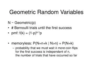
The Geometric Distribution • There are situations in which the goal is to obtain a fixed number of successes. • If the goal is to obtain one success, a random variable X can be defined that counts the number of trials needed to obtain that first success. • Geometric distribution – a distribution of a random variable that counts the number of trials needed to obtain a success.
Geometric Settings In a binomial setting, the number of trials n is fixed and the binomial random variable X counts the number of successes. In other situations, the goal is to repeat a chance behavior until a success occurs. These situations are called geometric settings. Definition: A geometric setting arises when we perform independent trials of the same chance process and record the number of trials until a particular outcome occurs. The four conditions for a geometric setting are • Binary? The possible outcomes of each trial can be classified as “success” or “failure.” B • Independent?Trials must be independent; that is, knowing the result of one trial must not have any effect on the result of any other trial. I T • Trials?The goal is to count the number of trials until the first success occurs. S • Success?On each trial, the probability p of success must be the same.
All four of these conditions must be met in order to use a geometric distribution. • Each observation falls into one of two categories: “success” or “failure” • The n observations are independent • The probability of success, call it p, is the same for each observation. • The variable of interest is the number of trials required to obtain the first success.
The Geometric Distribution • Let X = number of trials required for the first success • X is a geometric random variable • How is this distribution different than a binomial distribution?
Be aware of the key differences between binomial and geometric distributions. • Binomial: Finds the probability that k success will occur for in n number of attempts. • Geometric: Finds the probability that a success will occur for the first time on the nth try. • equation: P(x=n) = ( 1 - p )n-1 p
Is this a Geometric Setting? • A game consists of rolling a single die. The event of interest is rolling a 3; this event is called a success. The random variable is defined as X = the number of trials until a 3 occurs. Yes. Success = 3, Failure = any other number. p = 1/6 and is the same for all trials. The observations are independent. We roll until a 3 is obtained.
Geometric Setting? • Suppose you repeatedly draw cards without replacement from a deck of 52 cards until you draw an ace. There are two categories of interest: ace = success; not ace = failure. No. It fails the independence requirement. If the first card is not an ace then the 2nd card will have a greater chance of being an ace.
Using example 1, let’s calculate some probabilitiesA game consists of rolling a single die. The event of interest is rolling a 3; this event is called a success. The random variable is defined as X = the number of trials until a 3 occurs.
Example: The Birthday Game Read the activity on page 398. The random variable of interest in this game is Y = the number of guesses it takes to correctly identify the birth day of one of your teacher’s friends. What is the probability the first student guesses correctly? The second? Third? What is the probability the kth student guesses corrrectly? Verify that Y is a geometric random variable. B: Success = correct guess, Failure = incorrect guess I: The result of one student’s guess has no effect on the result of any other guess. T: We’re counting the number of guesses up to and including the first correct guess. S: On each trial, the probability of a correct guess is 1/7. Calculate P(Y = 1), P(Y = 2), P(Y = 3), and P(Y = k) Notice the pattern? Geometric Probability If Y has the geometric distribution with probability p of success on each trial, the possible values of Y are 1, 2, 3, … . If k is any one of these values,
Understanding Probability • In rolling a die, it is possible that you will have to roll the die many times before you roll a 3. • In fact, it is theoretically possible to roll the die forever without rolling a 3 (although the probability gets closer and closer to zero the longer you roll the die without getting a 3) • P(X = 50) = (5/6)49(1/6) = 0.0000
Probability distribution table for the geometric random variable never ends…. • This should remind you of an infinite geometric sequence from Algebra II • In order for it to be a true pdf, the sum of the second row must add up to 1.
Verifying it is a valid pdf • Recall the infinite sum formula: • In this case, a1 = p and r = 1 – p
Calculating Geometric Probabilities • P(X = k) = (1 – p)k – 1p • P(X =k) geometpdf (p, k) • “Probability that the first success occurs on the kth trial” • P(X < k) geometcdf (p, k)
The Expected Value • The mean or expected value of the geometric random variable is the expected number of trials needed for the first success. μ = 1/p
The formula for Standard Deviation of a Geometric series in not on the AP Statistics course syllabus. In case you are wondering, the formulas is: The variance of X is σ2 = (1 - p)/p2
The State Fair • Glenn likes the game at the state fair where you toss a coin into a saucer. You win if the coin comes to a rest in the saucer without sliding off. Glenn has played the game many times and has determined that on average he wins 1 out of every 12 times he plays. He believes that his chances of winning are the same for each toss. He has no reason to think that his tosses are not independent. Let X be the number of tosses until a win. Find his expected value.