Random Variables
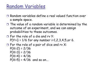
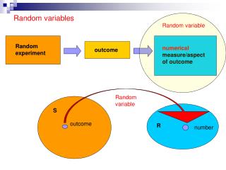
Random Variables. Random variables define a real valued function over a sample space. The value of a random variable is determined by the outcome of an experiment, and we can assign probabilities to these outcomes. For the role of a die and rv Y: P{Y=i} = 1/6 for any number i=1,2,3,4,5,or 6.

Random Variables
E N D
Presentation Transcript
Random Variables • Random variables define a real valued function over a sample space. • The value of a random variable is determined by the outcome of an experiment, and we can assign probabilities to these outcomes. • For the role of a die and rv Y:P{Y=i} = 1/6 for any number i=1,2,3,4,5,or 6. • For the role of a pair of dice and rv X:P{X=2} = 2/36P{X=3} = 2/36P{X=4} = 4/36P{X=5} = 4/36 and so on...
Bernoulli and Binomial RVs • Suppose a trial can be classified as either a success or failure (arrival of a packet or not). • For an rv X, let X=1 for an arrival, and X=0 for a non-arrival, and let p be the chance of an arrival. • p(0) = P{X=0} = 1 - pp(1) = P{X=1} = p • Suppose we had n trials. Then for a series of trials, define a binomial RV with parameters (n,p) as:
Poisson Random Variables • Poisson is an estimation of a binomial RV with params (n,p) • Let =np, therefore p= /n. • Remember that terms in box equal to about 1
Poisson RVs • In short, for poisson rv, we have the following distribution • The mean is • Take an interval [0,t] and N(t), the number of events occurring in that interval. • Without additional derivation, take it as true that • The number of events occurring in any fixed interval of length t is stated above. (It’s a Poisson random variable with parameter t and mean oft.)
Exponential RVs • The exponential rv arises in the modelling of the time between ocurrence of events. • Packet interarrival times • exponential rv X with parameter lambda: • The probability that this time exceeds h seconds • For a poisson random variable, the time between events is an exponentially distributed r.v.
... 0 T Relationship Between RVs • The number of trials (time units) until the arrival of a packet is a geomtric random variable. • As the number of trials gets large, the approaches an exponential random variable. • The interval [0,T] has been divided into n sub-intervals. • The number of packets arriving is a binomial random variable, • but with a large number of trials, can becomes a Poisson r.v. ... 0 T
The Big Black Box of delay(T seconds) Arriving customers Departing Customers Generic Delay Model
Some terms… • Each customer spends T seconds in the box, representing service time. • Let N(t) represent the number of customers in the system at timet. • Throughput: average number of messages per second that pass through the system.
Generic Delay Model N(t)= A(t) - D(t) A(t) The Big Black Box of delay(T seconds) Arriving customers Departing Customers D(t)
Arrivals • Let A(t) be the number of arrivals from time t=0 to time t. • Let D(t) be the number of departures. • Then number in system at time t: N(t) = A(t) - D(t).Assuming the system was empty at t=0.
Generic Delay Model N(t)= A(t) - D(t) A(t) The Big Black Box of delay(T seconds) Arriving customers Departing Customers D(t)
Let a1 be the 1st arrival in the system. The 2nd comes a2 time units later Num. of Customers in the system A(t) t a1 a2 a3 a4
Avg num in the system A(t) D(t) T4 T3 T2 T1 t a1 a2 a3 a4 • The number in the system at time t.
A(t) D(t) T4 T3 N(t) T2 T1 t a1 a2 a3 a4 Avg num in the system • The number in the system at time t.
Arrivals • Let a1 be the 1st arrival in the system. The 2nd comes a2 time units later. • Therefore the nth customer comes at time a1 + a2 + a3 + + an. • The avg arrival rate, , up to the time when the nth customer arrives is n / (a1 + a2 + + an) = customer/sec • Note the avg interarrival rate of customers is the reciprocal of : (a1 + a2 + + an) /n sec/customer • Arrival rate = 1/(mean of interarrival time).
Queuing fun • The long-term arrival rateis therefore customers/sec • Similarly, we can derive throughput Throughput = customers/sec Note the average service time is 1/.
Example • We are in line at the bank behind 10 people, and we estimate the teller taking around 5 minutes/per customer. • The throughput is the reciprocal of average time in service = 1/5 persons per minute • How long will we wait at the end of the queue? The queue size divided by the processing rate = 10/(1/5) = 50 minutes.
server queue Kendall Notation • Queuing systems are classified by a specific notation denoting: • The customer arrival pattern • The service time distribution • The number of servers • The maximum number of customers in the system. • E.g., M/M/1/Exponential interarrivals, exponential service times, 1 server, infinite buffer. (usually “M/M/1”) • M= exponential, D= deterministic, G= general • E.g., M/M/c/K exponenetial interarrivals, exponential service times, c servers, K customers can queue.
server queue M/M/1 Queue • In a steady state, i.e., <. • Interarrival time are random and have an exponential distribution. • FIFO servicing. • Service time is random and has an exponential distribution. • 1 server • No limit to the size of the queue.
M/M/1 Queue: busy period • Let’s derive traffic intensity . • Let P0be the probability of that the system is idle. • The system is defined to be in steady state, so what goes in must come out. = (0 customers)P0 + (1-P0) = (1-P0) P0 = 1 - (/) • The utilization is 1-P0 = (/) = • is in Erlang units and is a measure of traffic intensity.
M/M/1: Coming and Going • The interarrival times are exponential with mean ; We know the number of arrivals A(t) in an interval t is given by a Poisson random variable • It has a mean E[A(t)]= t • We can say the same of the departure times: they are exponential with a rate . The number of departures are a Poisson rv, the mean is E[D(t)]= t
More Derivation Fun • So what can we do with E[A(t)]= t and E[D(t)]= t? • With some derivation, we can figure out probabilities and expected means of • The mean number of customers in the system • The mean time customers spend in the system • The mean number queued up. • The mean time spent being queued up. • To do this we are going to set up a state diagram and solve for equations.
States • Let the “state” of our system be equal to the number of customers in the system. • Because we are modeling using Exponential RVs, the M/M/1 queue is memoryless. • The transition to a new state is independent of time spent in the current state, all that matters is the number in the system. • There is a certain probability of being in any state n. • In a steady state, this probability becomes independent of time and is written Pn. • Hence, that’s why we considered the idle time as P0.
Markovian Models • For any small interval of time t, there is a small chance of an arrival, and a small chance of a departure. • Let’s make t small enough that the chance of both a departure and arrival is negligible. t t 1 0 3 2 t t
t t t t ... n 2 n+1 1 n-1 0 t t t t States • For an arbitrary set of states, we have the following set of transition probabilities • Because we are in steady state, the flow between states (the transition probabilities) must balance. (Pn-1)t= (Pn)t
Transition Probabilities • Because we are in steady state, the flow between states (the transitions) must balance. (Pn+1)t= (Pn)t Pn+1 = / Pn Pn+1 = Pn • Let’s use this recurrence to solve for Pn.For n=1, P1=P0.For n=2, P2= P1 = 2P0Pn= nP0 • These probabilities must sum to 1…
Solving the Recurrence • Pn= nP0. These probabilities must sum to 1: and therefore and substituting above Pn= n(1- )
Mean number in system • What can we do with this? • It tells us the probability that there are n customers in the system. • Therefore, to find the mean number of customers in the system, it’s and substituting above Pn= n(1- )
Mean number of packets in the sys • What’s the mean number of packets in the system? • It’s the sum of the number of customers times the probability of that state.
Mean number in Queue • Notice the mean number in queue is larger than 1 even for the smallest traffic intensities. • And that the queue size tends towards infinity even though the service rate is larger than the arrival rate
Mean time in system • Call the mean time packets are in the system E[T]. • We know from Little’s Law that:E[N] = E[T] • Therefore,E[T] = E[N]/ = / (1- )
Meantime waiting in Queue • The mean time waiting in queue E[Q], is the time spent in the system not being serviced. • How long do we wait in service on average? • The reciprocal of the departure rate (1/ `.
Summary • E[N] = mean number in system • E[T] = mean time in system • = average arrival rate • avg number in system is equal to the avg number in queue and the avg number in service E[N] = E[Nq]+E[Ns] • Avg time in systems is equal to the avg time in queue and the avg time in service E[T] = E[Q]+E[X] • From Little’s Law that E[N] = E[T] • And E[Nq] = E[Q]
Summary • From Little’s Law that E[N] = E[T] • And E[Nq] = E[Q] • Given any one of E[N], E[Nq], E[T], or E[Q], we can calculate the other three; assuming we know and E[X]. • For example, if I tell you E[T], then E[N]= E[T], E[Q]= E[T]-E[X] E[Nq]= E[Q] = (E[T]-E[X])
Summary • We also know that E[N]= /(1- ) E[T] = E[N]/ = / (1- ) • We know that E[X] = 1/ = / • therefore E[T]= E[X]/(1- ) • and E[Q] = /(1- ) • and E[Q]= E[X]/(1- ) • E[Nq] = E[Q]= /(1- ) = 2/(1- )

