Binomial Random and Normal Random Variables
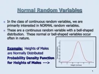
Binomial Random and Normal Random Variables. Lecture XI. Bernoulli Random Variables. The Bernoulli distribution characterizes the coin toss. Specifically, there are two events X =0,1 with X =1 occurring with probability p . The probability distribution function P [ X ] can be written as:.

Binomial Random and Normal Random Variables
E N D
Presentation Transcript
Binomial Random and Normal Random Variables Lecture XI
Bernoulli Random Variables • The Bernoulli distribution characterizes the coin toss. Specifically, there are two events X=0,1 with X=1 occurring with probability p. The probability distribution function P[X] can be written as: Lecture X
Sum of Two Bernoulli Variables • Next, we need to develop the probability of X+Y where both X and Y are identically distributed. If the two events are independent, the probability becomes: Lecture X
Transforming the Two Bernoulli Scenario • Now, this density function is only concerned with three outcomes Z=X+Y={0,1,2}. There is only one way each for Z=0 or Z=2. Specifically for Z=0, X=0 and Y=0. Similarly, for Z=2, X=1 and Y=1. However, for Z=1 either X=1 and Y=0 or X=0 or Y=1. Thus, we can derive: Lecture X
Expanding to Three Bernoulli Variables • Next we expand the distribution to three independent Bernoulli events where Z=W+X+Y={0,1,2,3}. Lecture X
Rewriting in Terms of Z • Again, there is only one way for Z=0 and Z=3. However, there are now three ways for Z=1 or Z=2. Specifically, Z=1 if W=1, X=1 or Y=1. In addition, Z=2 if W=1 and X=1, W=1 and Y=1, and X=1 and Y=1. Thus the general distribution function for Z can now be written as: Lecture X
Binomial Distribution • Based on this development, the binomial distribution can be generalized as the sum of n Bernoulli events. • For the case above, n=3. The distribution function (ignoring the constants) can be written as: Lecture X
Explaining the Constants • The next challenge is to explain the Crn term. To develop this consider the polynomial expression: Lecture X
Pascal’s Triangle • This sequence can be linked to our discussion of the Bernoulli system by letting a=p and b=(1-p). What is of primary interest is the sequence of constants. This sequence is usually referred to as Pascal’s Triangle: Lecture X
1 1 1 1 1 2 1 3 3 1 1 1 4 6 4 Lecture X
This series of numbers can be written as the combinatorial of n and r, or • Thus, any quadratic can be written as: Lecture X
As an aside, the quadratic form (a-b)n can be written as: Lecture X
Thus, the binomial distribution X~B(n,p) is then written as: Lecture X
Expected Value of Binomial • Next recalling Theorem 4.1.6: E[aX+bY]=aE[X]+bE[Y], the expectation of the binomial distribution function can be recovered from the Bernoulli distributions: Lecture X
Variance of Binomial • In addition, by Theorem 4.3.3: • Thus, variance of the binomial is simply the sum of the variances of the Bernoulli distributions or n times the variance of a single Bernoulli distribution Lecture X