GIS Lecture 11: Spatial Analyst
GIS Lecture 11: Spatial Analyst. Outline. Spatial Analyst Overview Grid Maps Raster Layers Raster Masks Kernel Density Smoothing Site Suitability Study Poverty Risk Model. Spatial Analyst Overview. Spatial Analyst. Traditional GIS Spatial queries, buffer analysis, overlay analysis

GIS Lecture 11: Spatial Analyst
E N D
Presentation Transcript
Outline • Spatial Analyst Overview • Grid Maps • Raster Layers • Raster Masks • Kernel Density Smoothing • Site Suitability Study • Poverty Risk Model
Spatial Analyst • Traditional GIS • Spatial queries, buffer analysis, overlay analysis • Spatial Analyst • Quantify spatial patterns and relationships • Track changes over time and determine patterns • Identify anomalous spatial patterns using mathematical statistics • Statistical significance and verifying conclusions
Primary Features • Data analysis • Allows rapid generation of maps that are based on complex statistics • Surface modeling • Creates predicted surface (grid maps) from unmeasured points based on statistical analysis of measured points
Load Spatial Analyst Extension • Tools, Extensions…
Grid Maps • Divides geographic space into uniform blocks called cells • Every cell represents a certain specified portion of the earth, such as a square mile, kilometer, meter, etc. • Each cell is given a value that describes the site, such as elevation, land use type, number of crimes, etc.
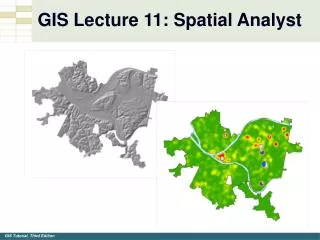
Grid Map Example • Housing units in City of Pittsburgh • Census Block Centroids • Kernel Density Raster Map
Raster Basemap • Free from U.S. Geological Survey (USGS) • Digital Elevation Model (DEM) • NED shaded relief, 1/3 arc second
Raster Basemap • Land use map • NLCD 2001
Raster Layer Properties • All raster maps are rectangular coordinate system
Create Raster Mask • Conversion Tools • Feature to Raster
Create Grid Map • Convert TIF to Grid • Export TIF
Environment Settings • Settings for environment tools • Set once to use throughout project
Extract Raster Masks • Extract (Clip) Land Use to Pgh Mask
Hillshade Raster • Hillshade function simulates illumination of a surface • Gives 3D appearance • Parameters • Altitude of light source above surface’s horizon • Angle (azimuth) relative to true north
Create Hillshade Raster • DEM to Hillshade
Resultant Hillshade Layer • Original hillshade layer Modified hillshade layer
Kernel Density Smoothing • Analyzes out of heart attack incidences in Pittsburgh • Uses point shapefile of census block centroids and point shapefile of out of hospital cardiac arrests (OHCA shapefile) • Estimates the incidence of heart attacks per unit area (density) • Two parameters • Cell size • Search radius
Existing Maps • OHCA and existing raster land use map • Heart attack locations are in developed areas
Existing Maps • Point centroids with population • OHCA points
Density Map • Create density map for heart attack incidence • Pittsburgh blocks average 300 ft per side in length • 2.5 blocks reasonable for defibrillator locations • Look at areas 5 blocks by 5 blocks or 1,500 ft • 150 ft cell size
Resultant Density Map • Shown with standard deviation and custom color ramp
Resultant Density Map • OHCA added • Note cluster in Downtown Pittsburgh where people work but don’t live
Raster Value Points • Extracts point estimates from raster surface for each OHCA point • Use extracted densities multiplied by block areas to estimate number of heart attacks • Better predictor of heart attacks
Extract Raster Value Points • Extraction Toolset
Resultant Layer • OHCAPredicted shapefile • Has attribute value, RASTERVALU, which is an estimate of heart attack density per sq foot, in the vicinity of each block
Calculate Predicted Heart Attacks • Resultant estimate will be larger than actual number of heart attacks in OCHA (these are only ones with bystander help) • Expression to calculate prediction • 5 * [RASTERVALU] * [AREA] • “five” is for 5 year sample of heart attack data in OHCA
Scatter Plot • Actual vs. predicted heart attacks • Pittsburgh has 7,466 blocks • 1,509 blocks with heart attacks
Resultant Graph • At the scale of blocks, predicted values correlate poorly with actual values • Factors other than population residence is needed
Site Suitability Study • Evaluates other factors for heart attack predictability (e.g. commercial land use) • Uses 600 foot buffer around commercial areas
Kernel Density Map • Create a kernel density map to use for calculations
Calculate Simple Query • Query kernel density map (HeartAttack) for areas that have high density and merit a defibrillator • 25 block area(1,500 ft x 1,500 ft , 2.25 x 10⁶ sq ft of area) • 10 or more heart attacks every 5 years in locations where bystander help is possible • Heart attack density : • 10 heart attacks/ 2.25 x 10⁶ sq ft =/0.000004444
Calculate Simple Query • Raster Calculator
Calculate Compound Query • Add second criteria: commercial buffer
Model for Risk Index • Poverty study as another risk for heart attacks • Population below poverty income line • Female headed household with children • Population with less than HS education • Workforce who are unemployed • Improper linear model for poverty • Calculate Z-score values • Data selected by subtracting the mean and dividing by the standard deviation for above variables, then averaging them
Risk Model Base Layers • Block Groups • NoHighSch2 (ho high school degree) • Male16Unem (males in workforce who are unemployed) • Poverty (population below poverty income) • Blocks • FHH (female headed households with children)
Risk Model Base Layers • Difficult to represent using vectors
Create New Model • New toolbox and model
Kernel Density Layers • Create kernel density layer for first input
Kernel Density Layers • Create kernel density layer for additional input
Standard Deviation Statistics • Mean and standard deviation for raster layers