Spatial Data Mining and Spatial Data Warehousing Special Topics In Database
Spatial Data Mining and Spatial Data Warehousing Special Topics In Database. Sadra Abedinzadeh Ashkan Zarnani Farzad Peyravi. Outline. Motivation and General Description Data Warehousing: Basic Concepts and Techniques Spatial Data Warehousing and Spatial OLAP Techniques

Spatial Data Mining and Spatial Data Warehousing Special Topics In Database
E N D
Presentation Transcript
Spatial Data Mining and Spatial Data WarehousingSpecial Topics In Database Sadra Abedinzadeh Ashkan Zarnani Farzad Peyravi
Outline • Motivation and General Description • Data Warehousing: Basic Concepts and Techniques • Spatial Data Warehousing and Spatial OLAP Techniques • Spatial Data Warehouse: Models and Construction • Spatial OLAP: Implementation and Application • Data Mining: Basic Concepts and Techniques • Spatial Data Mining • Mining Spatial Association Rules. • Spatial Classification and Prediction • Spatial Data Clustering Analysis • Conclusions and Future Research.
Motivation • Data warehousing: Integrating data from multiple sources into large warehouses and support on-line analytical processing and business decision making. • Data mining (knowledge discovery in databases): Extraction of interesting knowledge (rules, regularities, patterns, constraints) from data in large databases. • Necessity: Data explosion problem --- computerized data collection tools and mature database technology lead to tremendous amounts of data stored in databases. • We are drowning in data, but starving for knowledge!
Data Warehousing • “ A data warehouse is a subject-oriented, integrated, time-variant, and nonvolatile collection of data in support of management’s decision-making process.” --- W. H. Inmon • A data warehouse is • A decision support database that is maintained separately from the organization’s operational databases. • It integrates data from multiple heterogeneous sources to support the continuing need for structured and /or ad-hoc queries, analytical reporting, and decision support.
Modeling Data Warehouses • Modeling data warehouses: dimensions & measurements • Star schema: A single object (fact table) in the middle connected to a number of objects (dimension tables) radially. • Snowflake schema: A refinement of star schema where the dimensional hierarchy is represented explicitly by normalizing the dimension tables. • Fact constellations: Multiple fact tables share dimension tables. • Storage of selected summary tables: • Independent summary table storing pre-aggregated data, e.g., total sales by product by year. • Encoding aggregated tuples in the same fact table and the same dimension tables.
Example of Star Schema Time Dimension Table Sales Fact Table Product Dimension Table Many Time Attributes Time_Key Many Product Attributes Product_Key Store Dimension Table Location Dimension Table Store_Key Many Location Attributes Many Store Attributes Location_Key unit_sales dollar_sales Measurements Yen_sales
Example of a Snowflake Schema Supplier_Key Sales Fact Table Product Dimension Table Time Dimension Table Time_Key Supplier_Key Many Time Attributes Product_Key Product_Key Store_Key Store Dimension Table Location Dimension Table Location_Key Many Store Attributes Location_Key unit_sales Country dollar_sales Measurements Location_Key Yen_sales Region Location_Key
A Star-Net Query Model Customer Orders Shipping Method Customer CONTRACTS AIR-EXPRESS ORDER TRUCK PRODUCT LINE Time Product ANNUALY QTRLY DAILY PRODUCT ITEM PRODUCT GROUP DISTRICT SALES PERSON REGION DISTRICT COUNTRY DIVISION Geography Promotion Organization
All, All, All Construction of Data Cubes All Amount Comp_Method, B.C. Amount 0-20K 20-40K 40-60K 60K- sum Province B.C. Prairies Comp_Method Ontario sum Database Discipline … ... sum • Each dimension contains a hierarchy of values for one attribute • A cube cell stores aggregate values, e.g., count, sum, max, etc. • A “sum” cell stores dimension summation values. • Sparse-cube technology and MOLAP/ROLAP integration. • “Chunk”-based multi-way aggregation and single-pass computation.
Efficient Data Cube Computation Methods • Data cube can be viewed as a lattice of cuboids • The bottom-most cuboid is the base cube. • The top most cuboid contains only one cell. • Materialization of data cube • Materialize every (cuboid), none, or some. • Algorithms for selection of which cuboids to materialize. • Based on size, sharing, and access frequency. • Efficient cube computation methods • ROLAP algorithms. • Array-based cubing algorithm. ALL B A C AB BC AC ABC AC
OLAP: On-Line Analytical Processing • A multidimensional, LOGICAL view of the data. • Interactive analysis of the data: drill, pivot, slice_dice, filter. • Summarization and aggregations at every dimension intersection. • Retrieval and display of data in 2-D or 3-D crosstabs, charts, and graphs, with easy pivoting of the axes. • Analytical modeling: deriving ratios, variance, etc. and involving measurements or numerical data across many dimensions. • Forecasting, trend analysis, and statistical analysis. • Requirement: Quick response to OLAP queries.
OLAP Architecture • Logical architecture: • OLAP view: multidimensional and logic presentation of the data in the data warehouse/mart to the business user. • Data store technology: The technology options of how and where the data is stored. • Three services components: • data store services • OLAP services, and • user presentation services. • Two data store architectures: • Multidimensional data store: (MOLAP). • Relational data store: Relational OLAP (ROLAP).
Spatial Data Warehouse and Spatial OLAP • Spatial Data Warehouse: Integrated, subject-oriented, time-variant, and nonvolatile spatial data repository for data analysis and decision making. • Spatial Data Integration: A big issue. • Spatial data cube: Multidimensional spatial database. • Non-spatial dimensions: time, product, organization hierarchies. • Spatial dimensions: formed by geo-spatial hierarchies. • Non-spatial (numerical) measurements: • Distributive, algebraic, holistic. • Spatial Measurements: • Collection of spatial object pointers which may require spatial merge, overlay, or other operations.
Example: Weather Pattern Analysis • Input: • a map with about 3,000 weather probes scattered in B.C. • daily data for temperature, precipitation, wind velocity, etc. • concept hierarchies for all attributes • Output: • a map that reveals patterns: merged (similar) regions! • Goals: • interactive analysis (drill-down, slice, dice, pivot, roll-up) • fast response time • minimizing storage space used • Challenge: a merged region may contain hundreds of “primitive” regions (polygons).
Dimensions nonspatial (e.g. 25-30 degrees generalizes to hot) spatial-to-nonspatial (e.g. region “B.C.” generalizes to description “western provinces”) spatial-to-spatial (e.g. region “Burnaby” generalizes to region “Lower Mainland”) Measurements numerical distributive (e.g. count, sum) algebraic (e.g. average) holistic (e.g. median, rank) spatial collection of spatial pointers (e.g. pointers to all regions with 25-30 degrees in July) A Model of Spatial Data Warehouses
Star Model of a Spatial Data Warehouse • Dimensions • region_name • time • temperature • precipitation • Measurements • region_map • area • count Dimension table Fact table
Spatial Merge: Pre- vs On-line Computation Precomputing all: too much storage space On-line merge: very expensive
Spatial Measurements: Selective Materialization • Methods for computation of spatial measurements in spatial data cube. • Collect and store pointers to spatial objects in a spatial data cube:Computing on the fly --- expensive and slow. • Saving all the possible combinations --- huge space overhead. • Precompute and store rough approximations in a spatial data cube --- accuracy trade-off. • Selective computation: only materialize those which will be accessed frequently --- a reasonable choice. • Cube lattice and granularity of merge-able spatial objects. • Cuboid-level vs. cube cell level granularity.
Region_name Northern BC Interior BC Kooteney Lower Main. Vanc Isl. Okanagan cold mod warm hot Temperature Computing Spatial Measurements • Apply [HRU96] greedy algorithm to select cuboids • [HRU96] algorithm has granularity on a cuboid level • Finer granularity, on a cell level • Only selected cells are materialized (not the whole cuboid) • Factors in selections of cells • access frequency • size of a cell (number of merged objects) It could be better to save {1,3,4,7} than {1,3} • benefit for on-the-fly computation:If {1,3} is saved, it can be used for {1,3,6}. • Only neighboring objects are merged.
Integration of Data Mining and Data Warehousing • Data warehouse provides clean, integrated data for fruitful mining. • Data mining provides powerful tools for analysis of data stored in data warehouses. • OLAP can be viewed as data summarization and simple data mining. • Data mining provides more analysis tools, e.g., association, classification, clustering, pattern-directed, and trend analysis. • Mining multi-level knowledge by integration with OLAP facilities: mining in multiple data cubes.
Mining Different Kinds of Knowledge • Characterization: Generalize, summarize, and possibly contrast data characteristics, e.g., dry vs. wet regions. • Association: Rules like “inside(x, city) à near(x, highway)”. • Classification: Classify data based on the values in a classifying attribute, e.g., classify countries based on climate. • Clustering: Cluster data to form new classes, e.g., cluster houses to find distribution patterns. • Trend and deviation analysis: Find and characterize evolution trend, sequential patterns, similar sequences, and deviation data, e.g., housing market analysis. • Pattern-directed analysis: Find and characterize user-specified patterns in large databases, e.g., volcanos on Mars.
Different Mining Tasks in Spatial DBs • Spatial data mining tasks: • Spatial data characterization and comparison • Spatial clustering analysis • Spatial classification • Spatial association • Spatial pattern analysis • Spatial concept hierarchies: thematic vs. spatial. • Thematic hierarchy: e.g., agriculture (food (grain (corn, rice, ...), vegetable, fruit), others(...)). • Spatial hierarchy, based on • Spatial data structures (MBR, quad-tree & R-tree). • Spatial related semantics (geo-region classification). • Clustering analysis (e.g., neighborhood or adjacent_to).
A Geo-Spatial Data Mining Query Language: GMQL • Extension to Spatial SQL [Egenhofer’94]. • Support ad-hoc data mining queries. • mine characteristic rulestype of rule (characteristic, discriminant, association, clustering, classification)for “Description of states along I 80 highway” • from us_hiway, states_censusSQL like from, where clauses • where states_census.obj intersects us_hiway.objhigh level concepts andand highway = "I 80”spatial joins may be usedwith respect to states_census.obj, state_name, pop90, capita_incomelist of relevant attributes • set attribute threshold 51 for state_name thresholds for rules filtration
Background Knowledge for Data Mining • Conceptual "hierarchies" and generalization operators. • Instance-based: {freshman, ..., senior} Ì undergraduate. • Schema-based: address(city, province, country). • Rule-based: good(x) ¬ undergraduate(x)Ù gpa(x)³ 3.5. • Operation-based: aggregation, approximation, clustering, etc. • Where to get such background knowledge? • Implicitly stored in databases, such as address. • Explicitly defined by experts, such as "physics Ì science". • Formed with different attribute combinations, • food(category, brand, content _spec, package _size, price). • Generated automatically by data distribution analysis. • May need dynamic adjustment for a particular set of data. • Choose from multiple hierarchies or try them in parallel.
Automatic Generation of Numeric Hierarchies Count Amount 2000-97000 2000-16000 16000-97000 2000-12000 12000-16000 16000-23000 23000-97000
Spatial slicing Drilling-down on medium family income Spatial OLAP (Characterization) • Viewing data from different angles • Summarization on multiple concept levels
Mining Discriminant Rules • Discrimination: Comparison of two or more classes • Strategy: • Collect the relevant data respectively into the target class and the contrasting class • Generalize both classes to the same high level concepts, • Compare tuples with the same high level descriptions, • Present for every tuple its description and two numbers • support - distribution within single class • comparison - distribution between classes • Highlight the tuples with strong discriminant features • Interestingness: • Different measures of interestingness,e.g. consider also the sizes of different classes
Spatial OLAP (Comparison) • Comparing different classes of data Population increases faster in the western part. Drill down, and look at different dimensions to get explanation!!
Mining Association Rules • Association: Finding association among a set of attributes and their values. • Applications: pattern association, market analysis, etc. • Examples. • milk ® bread [5%, 60%] • tire Ù auto_accessories ® auto_services [2%, 80%] • Methods for mining associations : • Apriori ( Agrawal & Srikant’94) • Partition technique (Savasere, Omiecinski, Navathe’95) • Sampling (Toivonen’96)
Spatial Associations FIND SPATIAL ASSOCIATION RULE DESCRIBING "Golf Course" FROM Washington_Golf_courses, Washington WHERE CLOSE_TO(Washington_Golf_courses.Obj, Washington.Obj, "3 km") AND Washington.CFCC <> "D81" IN RELEVANCE TO Washington_Golf_courses.Obj, Washington.Obj, CFCC SET SUPPORT THRESHOLD 0.5
Spatial Associations & Hierarchy of Spatial Relationships • Spatial association: Association relationship containing spatial predicates, e.g., close_to, intersect, contains, etc. • Topological relations: • intersects, overlaps, disjoint, etc. • Spatial orientations: • left_of, west_of, under, etc. • Distance information: • close_to, within_distance, etc. • Hierarchy of spatial relationship: • “g_close_to”: near_by, touch, intersect, contain, etc. • First search for rough relationship and then refine it.
Efficient Mining of Spatial Associations • Two-step computation of spatial associations: • Step 1: rough spatial computation as a filter • MBR or R-tree rough estimation. • Step2: Detailed spatial algorithm as refinement • apply only to those pairs which have passed the rough spatial association testing (no less than min_support). • Multi-dimensional mining: • explore association relationships at any selected granularity level • perform drill-down and roll-up on any dimension.
Example: Spatial Association Rule Mining • “What kinds of spatial objects are close to each other in B.C.?” • Kinds of objects: cities, water, forests, usa_boundary, mines, etc. • Rules mined: • is_a(x, large_town) ^ intersect(x, highway) ® adjacent_to(x, water). [7%, 85%] • is_a(x, large_town) ^adjacent_to(x, georgia_strait) ® close_to(x, u.s.a.). [1%, 78%] • Mining method: Ariori + multi-level association + geo- spatial algorithms (from rough to high precision).
Data Classification • Data categorization based on a set of training objects. • Applications: credit approval, target marketing, medical diagnosis, treatment effectiveness analysis, etc. • Example: classify a set of diseases and provide the symptoms which describe each class or subclass. • The classification task: Based on the features present in the class_labeled training data, develop a description or model for each class. It is used for • classification of future test data, • better understanding of each class, and • prediction of certain properties and behaviors. • Data classification methods: Decision-trees (e.g., ID3, C4.5), statistics, neural networks, rough sets, etc.
A Decision-Tree Based Classification Method outlook sunny rain • A decision tree: • ID-3 and C4.5 (Quinlan’93): A top-down decision tree generation algorithm. • At start, all the training examples are at the root. • Partition examples recursively based on selected attributes. • Attribute selection: Maximizing an information gain measure, i.e., favoring the partitioning which makes the majority of examples belong to a single class. overcast humidity windy P N P N P
Scalable Classification Methods • Scalability of decision-tree classification algorithms. • Previous approaches: • Incremental tree construction (Quinlan’86): total cost is high. • Data sampling and discretizing continuous attributes (Cattlet’91): still in main memory. • Data partition and merge of parallel partition (Chan and Stolfo’91): reduced classification accuracy. • SLIQ & SPRINT (Mehta et al.’96, Shafer et al.’96): disk-based • Decision-tree construction algorithms. • Techniques: Pre-sorting, breadth_first tree-growing, and tree-pruning.
Generalization-Based Decision-Tree Induction • Integration of generalization with decision-tree induction. • Classification at primitive concept levels, e.g., precise temperature, humidity, outlook, etc. • Weakness: low-level concepts, scattered classes, bushy classification-trees, semantic interpretation problems. • Classification at high or medium concept levels: • may lead to imprecise classification. • Medium level generalization & adjustment: • Generalize to intermediate concept level(s). • Merge and split concept levels for better class representation and classification accuracy. • Efficiency: Analysis performed in compressed, generalized relations.
Mining Classification Rules • Classification: Based on the features present in the class_labeled training data, develop a description or model for each class. • Applications: credit approval, target marketing, medical diagnosis, treatment effectiveness analysis, etc. • Example: classify a set of diseases and provide the symptoms which describe each class or subclass.
Spatial Classification • Generalization-based induction • Interactive classification
Predictive Modeling in Databases • Predictive modeling: Predict data values or construct generalized linear models based on the database data. • One can only predict value ranges or category distributions. • Method outline: • Minimal generalization • Attribute relevance analysis • Generalized linear model construction • Prediction. • Determine the major factors which influence the prediction. • Data relevance analysis: uncertainty measurement, entropy analysis, expert judgement, etc. • Multi-level prediction: drill-down and roll-up analysis.
Spatial Prediction and Trend Analysis • Spatial trend predictive modeling (Ester et al’97): • Discover centers: local maximal of some non-spatial attribute. • Determine the (theoretical) trend of some non-spatial attribute, when moving away from the centers. • Discover deviations (from the theoretical trend). • Explain the deviations. • Example: Trend of unemployment rate change according to the distance to Munich. • Similar modeling can be used to study trend of temperature with the altitude, degree of pollution in relevance to the regions of population density, etc.
Data Clustering Analysis • Data clustering (“unsupervised learning”): Cluster objects into classes, based on their features, which maximize intraclass similarity and minimize interclass similarity. • Probability-based vs. distance-based clustering analysis. • Typical probability-based clustering analysis algorithms: • COBWEB (Fisher’87): Incremental concept formation. • Category utility measurement (probability of each concept’s occurrence) • Top-down, incremental, hierarchical organization of concepts. • CLASSIT (Gennari’89): extend it to real-valued data. • Typical distance-based clustering analysis algorithms: • Statistics-based, k-means, k-medoids, nearest neighbors.
Distance-Based Spatial Clustering Analysis • Statistical approaches: scan data frequently, iterative optimization, hierarchical clustering, etc. • CLARANS (Ng & Han’94): randomized search (sampling) + PAM (a distance-based clustering algorithm). • DASCAN (Ester et al.’96): density-based clustering using spatial data structures (R*-tree). • BIRCH (Zhang et al.’96): Balanced iterative reducing and clustering using hierarchies. • Focus on densely occupied portions of the data space. • Measurement reflects the “natural” closeness of points. • A height-balanced tree (CF-tree) is used for clustering. • Describe aggregate proximity relationships (Knorr & Ng’96).
Spatial Clustering • How can we cluster points? • What are the distinct features of the clusters? There are more customers with university degrees in clusters located in the West. Thus, we can use different marketing strategies!
Data and Knowledge Visualization • Visualization of characteristic and discriminant rules: • tables & cubes + bar/pie charts, curves, surfaces, etc. • Visualization of association rules: • Association rule graph: Nodes for large 1-itemset, lines for large 2-items sets, arrows for implication strength. • Association matrix: support/confidence: size/color in cells. • Cluster analysis: viewing clusters and their characteristics. • Classification: colored decision trees. • Prediction: curves, pie charts, and relevance analysis results. • Deviation analysis: boxplots (quartiles, median) and outliers. • Visual impression of large data mining results • arrange and color data items as pixels (Keim et al.’94)
Visual Data Mining (ref. D. Keim SIGMOD’96 Tutorial) • Data visualization and exploratory analysis: • Interactive, usually undirected search for structures, trends, etc. • Typical data visualization techniques: • Geometric techniques, icon-based techniques, pixel-oriented techniques, hierarchical techniques, graph-based techniques, 3D-techniques, dynamic techniques, and hybrid techniques. • Database visualization systems: • Statistics-oriented systems, visualization-oriented systems, database-oriented systems and special purpose systems. • Visual database exploration is another powerful approach to data mining, especially spatial data mining.
Data Mining Interfaces • Interactive mining versus a data mining language. • Specification of data mining tasks. • Data sets: any sets of data in databases • Mining task specification: kinds of knowledge or forms of rules to be mined. • Background knowledge (e.g., concept hierarchies): specification and manipulation. • Interestingness measurement: significance, confidence, thresholds, concept levels, etc. • Transformation and manipulation of output results. • Roll-up vs. drill-down. • Multiple output forms: generalized relations, crosstabs, charts, curves, and other visual outputs.
Systems for Data Warehousing and Data Mining • Systems for Data Warehousing • Arbor Software: Essbase • Oracle (IRI): Express • Cognos: PowerPlay • Redbrick Systems: Redbrick Warehouse • Microstrategy: DSS/Server • Systems or Research Prototypes for Data Mining • IBM: QUEST (Intelligent Miner) • Silicon Graphics: MineSet • Integral Solutions Ltd.: Clementine • Information Discovery Inc.: Data Mining Suite • SFU (DBTech): DBMiner, GeoMiner • Rutger: DataMine, GMD: Explora, U Munich: VisDB
Conclusions • Data warehousing and data mining: • A rich, promising, young field with broad applications and many challenging research issues. • Imminent task: spatial database analysis --- from spatial data manipulation to on-line spatial analytical processing (Spatial OLAP) and spatial data mining. • Spatial data cube construction: fine granularity analysis. • Multiple spatial data mining tasks: Characterization, association, classification, clustering, sequence and pattern analysis, prediction, etc. • Integration of data mining with OLAP: OLAP-based spatial data mining. • Integration of spatial analysis methods, spatial query processing methods, and spatial indexing techniques.