Download
1 / 24
240 likes | 306 Views
Explore advanced econometric techniques, such as modeling wages and income inequality, through theoretical frameworks and empirical applications. Develop skills in regression models, time series analysis, and structural modeling.

E N D
Introduction Econometrics forMathematics Bachelor Students Kees Jan van Garderen Programme Director BSc & MSc in Econometrics
Kees Jan van GarderenProgramme Director BSc & MSc in Econometrics • BSc& MSc in Econometrics UvA, MSc title: • Fractionele Matrix CalculusPhD, Trinity College, Cambridge, title: • Inference in Curved Exponential Modelsuses non-Riemannian geometry in econometric/statistical models • Research Interest : Econometrics • Econometric Theory - Exact Distribution Theory • Approximations (Tilted or Saddlepoint, Edgeworth ) • Inference and Curvature in Econometric Models • Income Inequality • Aggregation • Teaching • 2nd year Econometrics 1 and 2 • M.Phil. Tinbergen Institute, Advanced Econometrics II
Department of Quantitative Economics • Actuarial Science • Operations Research • Econometrics & Economic Theory (Mathematical Economics) • UvA - Econometrics • CeNDEF(Center for Nonlinear Dynamics in Economics and Finance)
Econometrics and Statistics • Regression Models • Linear & non-Linear • Multivariate Analysis • Cross-section • Likelihood Theory • Time Series • ARIMA • Non-Parametrics
Econometrics and Statistics • Non Experimental (i.i.d) Data • sample selection (self-selection) • endogeneity, instrumental variables • Misspecified Models : diagnostics/ model choice • Structural Modelling • causal relationships : economic theory and insight • Identification : Structural <==> Reduced Form • moment conditions • Multivariate Time-series Analysis VAR with Non-stationary data Cointegration CVAR
Three Examples • Modelling wages • Instrumental Variable regression • Heckman • Demand and Supply • Cointegration (modelling with non-stationary timeseries)
Modelling Wages I : returns to schooling • Log(income) = b1 + b2schooling + b3 age + b4 tenure +…+ e • E-views Expected income determines length of schooling People with high academic ability earn more and will go to school longer (pay-offs for them are higher) Inappropriate to attribute to schooling only.
Regression with Instrumental Variables Model Estimator (OLS) Unbiased? Consistent? Model Stochastics Gewone Kleinste Kwadraten (via regressie of lineaire algebra)
Modelling Wages II : sex discrimination • Log(income) = b1 + b2 Male + b3 age + …. + e1 • . reg LGEARNCL COLLYEAR EXP ASVABC MALE ETHBLACK ETHHISP • ------------------------------------------------------ • LGEARNCL | Coef. Std. Err. t P>|t| • -------------+---------------------------------------- • COLLYEAR | .1380715 .0201347 6.86 0.000 • EXP | .039627 .0085445 4.64 0.000 • ASVABC | .0063027 .0052975 1.19 0.235 • MALE | .3497084 .0673316 5.19 0.000 • ETHBLACK | -.0683754 .1354179 -0.50 0.614 • ETHHISP | -.0410075 .1441328 -0.28 0.776 • _cons | 1.369946 .2884302 4.75 0.000 • ------------------------------------------------------
Modelling Wages II • Log(income) = b1 + b2 Male + b3 age + …. + e1 • Working = 1 : Z* > 0 = 0 : Z* 0 • Z* = f( predicted earnings, children, married, ) + e2If e1 and e2 correlated, then E[ e1 | working ] 0
Maximum Likelihood • . g COLLYEAR = 0 • . replace COLLYEAR = S-12 if S>12 • (286 real changes made) • . g LGEARNCL = LGEARN if COLLYEAR>0 • (254 missing values generated) • . heckman LGEARNCL COLLYEAR EXP ASVABC MALE ETHBLACK ETHHISP, select(ASVABC MALE ETHBLACK ETHHISP SM SF SIBLINGS) • Iteration 0: log likelihood = -510.46251 • Iteration 1: log likelihood = -509.65904 • Iteration 2: log likelihood = -509.19041 • Iteration 3: log likelihood = -509.18587 • Iteration 4: log likelihood = -509.18587 • Heckman selection model Number of obs = 540 • (regression model with sample selection) Censored obs = 254 • Uncensored obs = 286 • Wald chi2(6) = 95.83 • Log likelihood = -509.1859 Prob > chi2 = 0.0000
Maximum Likelihood • ------------------------------------------------------------------------------ • | Coef. Std. Err. z P>|z| [95% Conf. Interval] • -------------+---------------------------------------------------------------- • LGEARNCL | • COLLYEAR | .126778 .0196862 6.44 0.000 .0881937 .1653623 • EXP | .0390787 .008101 4.82 0.000 .023201 .0549565 • ASVABC | -.0136364 .0069683 -1.96 0.050 -.027294 .0000211 • MALE | .4363839 .0738408 5.91 0.000 .2916586 .5811092 • ETHBLACK | -.1948981 .1436681 -1.36 0.175 -.4764825 .0866862 • ETHHISP | -.2089203 .159384 -1.31 0.190 -.5213072 .1034667 • _cons | 2.7604 .4290092 6.43 0.000 1.919557 3.601242 • -------------+---------------------------------------------------------------- • select | • ASVABC | .070927 .008141 8.71 0.000 .054971 .086883 • MALE | -.3814199 .1228135 -3.11 0.002 -.6221298 -.1407099 • ETHBLACK | .433228 .2184279 1.98 0.047 .0051172 .8613388 • ETHHISP | 1.198633 .299503 4.00 0.000 .6116179 1.785648 • SM | .0342841 .0302181 1.13 0.257 -.0249424 .0935106 • SF | .0816985 .021064 3.88 0.000 .0404138 .1229832 • SIBLINGS | -.0376608 .0296495 -1.27 0.204 -.0957729 .0204512 • _cons | -4.716724 .5139176 -9.18 0.000 -5.723984 -3.709464 • -------------+---------------------------------------------------------------- • /athrho | -.9519231 .2430548 -3.92 0.000 -1.428302 -.4755444 • /lnsigma | -.4828234 .0727331 -6.64 0.000 -.6253776 -.3402692 • -------------+---------------------------------------------------------------- • rho | -.7406524 .1097232 -.8913181 -.4426682 • sigma | .6170388 .0448791 .5350593 .7115788 • lambda | -.4570113 .0967091 -.6465576 -.267465 • ------------------------------------------------------------------------------ • LR test of indep. eqns. (rho = 0): chi2(1) = 7.63 Prob > chi2 = 0.0058 • ------------------------------------------------------------------------------
Maximum Likelihood versus Linear regression • . heckman LGEARNCL COLLYEAR EXP ASVABC MALE ETHBLACK ETHHISP, • select(ASVABC MALE ETHBLACK ETHHISP SM SF SIBLINGS) • ------------------------------------------------------------------------------ • | Coef. Std. Err. z P>|z| [95% Conf. Interval] • -------------+---------------------------------------------------------------- • LGEARNCL | • COLLYEAR | .126778 .0196862 6.44 0.000 .0881937 .1653623 • EXP | .0390787 .008101 4.82 0.000 .023201 .0549565 • ASVABC | -.0136364 .0069683 -1.96 0.050 -.027294 .0000211 • MALE | .4363839 .0738408 5.91 0.000 .2916586 .5811092 • ETHBLACK | -.1948981 .1436681 -1.36 0.175 -.4764825 .0866862 • ETHHISP | -.2089203 .159384 -1.31 0.190 -.5213072 .1034667 • _cons | 2.7604 .4290092 6.43 0.000 1.919557 3.601242 • -------------+---------------------------------------------------------------- • . reg LGEARNCL COLLYEAR EXP ASVABC MALE ETHBLACK ETHHISP • ------------------------------------------------------------------------------ • LGEARNCL | Coef. Std. Err. t P>|t| [95% Conf. Interval] • -------------+---------------------------------------------------------------- • COLLYEAR | .1380715 .0201347 6.86 0.000 .0984362 .1777068 • EXP | .039627 .0085445 4.64 0.000 .022807 .0564469 • ASVABC | .0063027 .0052975 1.19 0.235 -.0041254 .0167309 • MALE | .3497084 .0673316 5.19 0.000 .217166 .4822509 • ETHBLACK | -.0683754 .1354179 -0.50 0.614 -.334946 .1981952 • ETHHISP | -.0410075 .1441328 -0.28 0.776 -.3247333 .2427183 • _cons | 1.369946 .2884302 4.75 0.000 .8021698 1.937721 • ------------------------------------------------------------------------------
Demand and Supply • Q = 5 - 0.9 P + 1.0 income + e1 ( demand ) • Q : Quantity (in kg), • P : Price (in €) • income in ‘000 € • e~ N( 0, S ). Q = 3 + 1.5 P – 1.0 cost + e2 ( supply ) cost in ‘000 €.
Increase cost Increase cost & inc at random Q 12 solutions 10 8 6 4 2 P 2 4 6 8 10 12 Demand and Supply(unconventionally P(rices) on horizontal axis) Shift in supply supply demand demand Increase income supply demand
Varying Cost only Instrumental Variable estimation Data : Price & Quantity Varying income Q 12 supply 10 8 6 4 2 demand P 2 4 6 8 10 12
True relations Q = 3 + 1.5 P – 1.0 cost + e2 ( supply ) Estimated relations • Q = 5 - 0.9 P + 1.0 income + e1 ( demand ) • We can : • Estimate 2 equations correctly from 1 set of data • Lesson: • Running regression can be very misleading • Use economic theory and econometric techniques
Cointegration : Money demand • m-p = g + g2 y +g3Dp + g4 R • m -p : real money balances in logs, y : real transactions (i.e.GDP) in logs, p : log price index,R : interest rate • GDP90 : GDP(A) at current market prices index (1990=100) • P : RPI: Retail price index all items (1985=100) • M4 : Money stock M4 (end period) : level, Seasonally Adjusted R : Treasury Bills 3 month yield • Q1,...,Q4: Quarter 1 to quarter 4 dummy.
Possibilities • Minor Econometrics • Deficiency Programme/Schakel programma • B.Sc. in Econometrics and ORM or Actuarial Sciences • M.Sc. in Econometrics (Financial Econometrics, Math Econ)
M.Sc. Econometrics /Mathematical Economics • Blok I (15 EC) • Adv Econometrics 1 • General Equilibrium Th. • Elective • Blok II (15 EC) • Adv. Econometrics 2 • Game Theory • Elective • Blok III (15 EC) • Field course (Fin. Ectr) • Field course (Micr. Ectr) • Field course (caput ME2) • Blok IV • Master Thesis
Deficiëntieprogramma Econometrie (35 ec) studenten met WO bachelor- of master Wiskundeof Natuurkunde of equivalente exacte opleiding • … alvorens toegelaten te kunnen worden tot de MSc in Econometrics, de volgende deficiënties weggewerkt te hebben: • steunvakken KReS 3 (5 ec) en KReS 4 (5 ec) • verbredingsvak Econometrie 3 (5 ec) • verbredingsvak Tijdreeksanalyse (5 ec) • verbredingsvak Wiskundige Economie B (5 ec) • Wiskundige Economie A (5 ec) en Inleiding Speltheorie (5 ec)
Tot spoedig ziens !? • Kees Jan van Garderen • Programme Director BSc & MSc Econometrics • Faculty of Economics and Business • University of Amsterdam • Roetersstraat 11 • 1018 WB, Amsterdam • Room E 3.25, Economics Building • E-Building, central tower • http://www.studeren.uva.nl/msc_econometrics • http://studiegids.uva.nl/web/uva/sgs/en/p/241.html • tel +31-20-525 4220 • fax +31-20-525 4349 • K.J.vanGarderen@uva.nl