Introduction to Econometrics

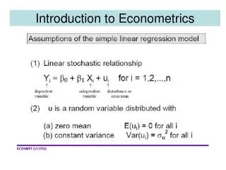
Introduction to Econometrics Lecture 7 Heteroskedasticity and some further diagnostic testing

Topics to be covered • Heteroskedasticity • Some further diagnostic testing • Normality of the disturbances • Multicollinearity

Econometric problems

Heteroskedasticity What does it mean? The variance of the error term is not constant What are its consequences?The least squares results are no longer efficient and t tests and F tests results may be misleading How can you detect the problem?Plot the residuals against each of the regressors or use one of the more formal tests How can I remedy the problem? Respecify the model – look for other missing variables; perhaps take logs or choose some other appropriate functional form; or make sure relevant variables are expressed “per capita”

Consumption function example (cross-section data): credit worthiness as a missing variable?

The Homoskedastic Case

The Heteroskedastic Case

The consequences of heteroskedasticity • OLS estimators are still unbiased (unless there are also omitted variables) • However OLS estimators are no longer efficientor minimum variance • The formulae used to estimate the coefficient standard errors are no longer correct • so the t-tests will be misleading (if the error variance is positively related to an independent variable then the estimated standard errors are biased downwards and hence the t-values will be inflated) • confidence intervals based on these standard errors will be wrong

Detecting heteroskedasticity • Visual inspection of scatter diagram or the residuals • Goldfeld-Quandt test • suitable for a simple form of heteroskedasticity • Breusch-Pagan test • a test of more general forms of heteroskedastcity

Residual plots Plot residuals against one variable at a time

Goldfeld-Quandt test (JASA, 1965) • Suppose it looks as ifsui = suXi i.e. the error variance is proportional to the square of one of the X’s • Rank the data according to the culprit variable and conduct an F test using RSS2/RSS1 where these RSS are based on regressions using the first and last [n-c]/2 observations [c is a central section of data usually about 25% of n] • Reject H0 of homoskedasticity if Fcal > Ftables

Breusch-Pagan test • Regress the squared residuals on a constant, the original regressors, the original regressors squared and, if enough data, the cross-products of the Xs • The null hypothesis of no heteroskedasticity will be rejected if the value of the test statistic is “too high” (P-value too low) • Both c2 and F forms are available in PcGive

Remedies • Respecification of the model • Include relevant omitted variable(s) • Express model in log-linear form or some other appropriate functional form • Express variables in per capita form • Where respecification won’t solve the problem use robust Heteroskedastic Consistent Standard Errors (due to Hal White, Econometrica 1980)

ARCH • Note: with time series data, particularly high-frequency data (for example daily or hourly financial data) a special form of heteroskedasticity called Autoregressive Conditional Heteroskedasticty (ARCH) may be present • We can see it graphically as excessive volatility of the time series in certain short bursts • I will say more about this when we look in more detail at dynamic models

Normality of the disturbances • Test null hypothesis of normality • Use 2 test with 2 degrees of freedom • At 5% level reject H0 if 2 > 5.99 • non-normality may reflect outliers or a skewed distribution of residuals

Reset test • originated by Ramsey (1969) • tests for functional form mis-specification • run regression and get fitted values • now regress Y on X’s and powers of fitted Ys • if these additional regressors are significant (judged by F test) then the original model is mis-specified

Multicollinearity What does it mean? A high degree of correlation amongst the explanatory variables What are its consequences?It may be difficult to separate out the effects of the individual regressors. Standard errors may be overestimated and t-values depressed. Note: a symptom may be high R2 but low t-values How can you detect the problem?Examine the correlation matrix of regressors - also carry out auxiliary regressions amongst the regressors. Look at the Variance Inflation Factors • NOTE: • be careful not to apply t tests mechanically without checking for multicollinearity • multicollinearity is a data problem, not a misspecification problem

Variance Inflation Factor (VIF) Multicollinearity inflates the variance of an estimator VIFJ = 1/(1-RJ2) where RJ2 measures the R2 from a regression of Xj on the other X variable/s serious multicollinearity problem if VIFJ>5

Introduction to Econometrics