Introduction to Econometrics
Introduction to Econometrics. What do I expect of you before you come to class? Print out the slides. Read the chapter, and as you read, write questions down on the slides. Therefore, when I am lecturing, I do not expect it to be the first time you are hearing about a concept.

Introduction to Econometrics
E N D
Presentation Transcript
Introduction to Econometrics • What do I expect of you before you come to class? • Print out the slides. • Read the chapter, and as you read, write questions down on the slides. • Therefore, when I am lecturing, I do not expect it to be the first time you are hearing about a concept. • If you don’t do this, it will seem like I am going really, really fast. • If this approach to my teaching/your learning, which places high demand on your pre-class preparation, doesn’t suit you, I won’t be offended if you take Eco205 from someone else.
Brief Overview of the Course • Economic theory often suggests the sign of important relationships, often with policy implications, but rarely suggests quantitative magnitudes of causal effects. • What is the quantitative effect of reducing class size on student achievement? Expected sign is ? • How does another year of education change earnings? • What is the effect on output growth of a 1 percentage point decrease in interest rates by the Fed? • What is the effect on housing prices of environmental improvements?
This course is about using data to measure causal effects. • Typically only have observational (nonexperimental) data • level of education vs. wages • cigarette price vs. quantity demanded • selectivity of a college vs. wages • class size vs. test scores • democracy measure vs. GDP per capita (income) • Difficulties arise from using observational data to estimate causal effects • confounding effects (omitted factors) • simultaneous causality • Remember, correlation does not imply causation ! • Randomized experiments often not feasible
Review of Probability and Statistics(SW Chapters 2, 3) • Empirical problem: Class size and educational output • Policy question: What is the effect on test scores (or some other outcome measure) of reducing class size by one student per class? By 8 students/class?
Initial look at the data(You should already know how to interpret this table) • What do we learn about the relationship between test scores and the STR?
Do districts with smaller classes have higher test scores? STR
Compare districts with “small” (STR < 20) and “large” (STR ≥ 20) class sizes 1. Estimation of = population difference between group means 2. Test the hypothesis that = 0 3. Construct a confidence interval for
1. Estimation • Is this a large difference in a real-world sense? • Standard deviation across districts = 19.1 • Difference between 60th and 75th percentiles of test score distribution is 667.6 – 659.4 = 8.2 • Is this a big enough difference to be important for school reform discussions, for parents, for a school committee?
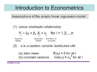
(a) Population, random variable, and distribution • Population • The group or collection of all possible entities of interest (school districts) • We will think of populations as infinitely large • Random variable Y • Numerical summary of a random outcome (district average test score, district STR) • Population distribution • Gives the probabilities of different values of Y • when Y is discrete, Pr[Y = 650] • when Y is continuous, Pr[640 ≤ Y ≤ 660]
Two Random Variables • Two random variables have a joint distribution • cov(X,Z) = E[(X – X)(Z – Z)] = XZ • Linear association • Units? • If X and Z are independently distributed, then cov(X,Z) = 0 (but not vice versa!!) • cov(X,X) = E[(X – X)(X – X)] = E[(X – X)2]
Covariance is negative so is the correlation…
(c) Conditional distributions • Conditional distributions • distribution of test scores, given that STR < 20 • Conditional moments • conditional mean is written E(Y|X = x) • E(Test scores|STR < 20) • note that the prob here = (1/ns) for the test scores, yielding the average test score among small districts • conditional variance is written Var(Y|X=x) • Var(Test scores|STR < 20)
Examples of Conditional Mean • Wages of all female workers (Y = wages, X = gender) • Mortality rate of patients given an experimental treatment (Y = live/die; X = treated/not treated) • The difference in means from the t-test • = E(Test scores|STR < 20) – E(Test scores|STR ≥ 20)
Properties of Conditional Mean • Law of Iterated Expectations E[Y] = E[ E[Y|X] ] • Recall that • And expected value of E[Y|X] is • Note that y takes on k outcomes, x takes on l outcomes
L.I.E. example • Consider the following joint probability distribution table for two random variables, the number of children a household has (C) and the location of the household (L). • Number of Children (C) • Location (L) 0 1 2 3 • West (L = 0) 0.10 0.05 0.10 0.05 • Central (L = 1) 0.10 0.02 0.10 0.02 • East (L = 2) 0.15 0.18 0.10 0.03 • Show that L.I.E. holds
Properties of Conditional Mean • If E(X|Z) = X, then corr(X,Z) = 0 (not necessarily vice versa) • Proof: Assume X = 0 and Z = 0 for simplicity • First, note that corr(X, Z) = 0 implies cov(X,Z) = 0. Why? • Start with definition of cov(X,Z) …
(d) Distribution of a sample of data drawn randomly from a population: Y1,…, Yn • The data set is (Y1, Y2, … , Yn), where Yi = value of Y for the ith individual (district, entity) sampled • Yiare said to be i.i.d. “independent and identically distributed”
Mathematics of Expectations • Read Appendix 2.1 carefully • Let’s prove this one, for practice
3. Hypothesis Testing • H0: Y= Y,0 vs. H1: Y> Y,0 , < Y,0 , ≠ Y,0 • p-value= probability of drawing a statistic at least as adverse to H0 as the value actually computed with your data, assuming that H0 is true. • “lowest significance level at which you can reject H0” • The significance level of a test is a pre-specified probability of incorrectly rejecting H0, when H0is true.
Comments on the Student t-distribution • Astounding result really … if Yi are i.i.d. normal, then you can know the exact, finite-sample distribution of the t-statistic … it’s the Student’s t-distribution. • tn-1 approaches z“quickly” as n increases • t30,.05=2.042, t60,.05=2.000, t100,.05=1.983 • Requires the impractical assumption that population distribution of X is normal
Comments on Student t distribution 4. Consider the statistic to test difference in means between 2 groups (s,l): It does not have an exact t-distribution in small samples, even if Y is normally distributed. This statistic does though (when Y normal), but only if Bottom line: That’s not likely, so pooled std error formula usually inappropriate. So use different-variance formula with large-sample z critical values.
Confidence Intervals A 95% confidence intervalfor Y is an interval that is expected to contain the true value of Y in 95% of repeated samples of size n. Note: What is random here?