Appendix D: Application of Genetic Algorithm in Classification
This document explores the application of Genetic Algorithms (GAs) in classification tasks, particularly focusing on decision tree algorithms like ID3 and C4.5. It discusses how decision trees generate classification rules in the IF-THEN format, which enhances interpretability. The paper goes on to define GAs for classification rule discovery, with individuals represented as bit strings encoding rules. It elaborates on genetic operations like generalization and specialization to optimize rule creation, and details the fitness functions used to evaluate rule performance based on predictive accuracy and completeness.

Appendix D: Application of Genetic Algorithm in Classification
E N D
Presentation Transcript
Appendix D: Application of Genetic Algorithm in Classification Duong Tuan Anh 5/2014
Classification with Decision trees Training data Class No No Yes Yes Yes No Yes No Yes Yes Yes Yes Yes No
Decision tree There exists the algorithm to create a decision tree from the training set (ID3, C4.5)
Classification rules from decision tree • Represent the knowledge in the form of IF-THEN rules • One rule is created for each path from the root to a leaf • Each attribute-value pair along a path forms a conjunction • The leaf node holds the class prediction • Rules are easier for humans to understand. Example IF age = “<=30” AND student = “no” THEN buys_computer = “no” IF age = “<=30” AND student = “yes” THEN buys_computer = “yes” IF age = “31…40” THEN buys_computer = “yes” IF age = “>40” AND credit_rating = “excellent” THEN buys_computer = “no” IF age = “>40” AND credit_rating = “fair” THEN buys_computer = “yes”
GA for classification rule discovery • Individual representation • Each individual encodes a single classification rule • Each rule is represented as a bit string • Example: Instances in the training set are describe by two Boolean attributes A1 and A2 and two classes: C1 and C2 • Rule: IF A1 AND NOT A2 THEN C2 bit string “100” • Rule: IF NOT A2 AND NOT A2 THEN C1 bit string “001” • If the attribute has k values, k > 2 then k bits are used to encode the attribute values. Classes can be encoded in a similar fashion.
Genetic operators for rule discovery • Generalizing/Specializing Crossover • Overfitting: a situation in which a rule is covering one training example. generalization • Underfitting: a situation in which a rule is covering too many training examples. specialization • The generalizing/specialization crossover operators can be implemented as the logical OR and AND, respectively. • Example: Two crossover points children produced by children produced by Parents generalization crossover specialization crossover 0 | 1 0 | 1 0 | 1 1 | 1 0 | 0 0 | 1 1 | 0 1 | 0 1 | 1 1 | 0 1 | 0 0 | 0 OR AND
Fitness function • Let a rule be of the form: IF A THEN C where A is the antecedent and C is the predicted class. Predictive accuracy of a rule called confidence factor (CF) is defined: CF = |A C|/|A| |A|: the number of examples satisfying all the conditions in the antecedent A |A C|: the number of examples that both satisfy the antecedent A and have the class predicted by the consequent C. Example: A rule covers 10 examples (i.e. |A| = 10), in which 8 examples have the class predicted by the rule (i.e. |A & C| = 8), then CF of the rule is CF = 80%. • The performance of a rule can be summarized by a matrix called a confusion matrix.
Confusion matrix TP = True positives = Number of examples satisfying A and C FP = False positives = Number of examples satisfying A but not C FN = False negatives = Number of examples not satisfying A but satisfying C TN = True negatives = Number of examples not satisfying A nor C CF measure is defined in terms of the above notation: CF = TP/(TP + FP).
Fitness function (cont.) • We can know measure the predictive measure of a rule by taking into account not only its CF but also a measure of how “complete” a rule is. • Completeness of the rule: what is the proportion of examples having the predicted class C that is actually covered by the rule antecedent. • The rule completeness measure: Comp = TP/(TP+FN) • The fitness function combines the CF and Comp measures: Fitness = CF Comp. • An initial population is created consisting of randomly generated rules. • The process of generating a new population based on prior populations of rules continues until a population, P, evolves where each rule in P satisfies a prespecified fitness threshold.
Reference • A. A. Freitas, A Survey of Evolutionary Algorithms for Data Mining and Knowledge, in: Advances in Evolutionary Computing, Springer, 2003.