Download
1 / 100
1k likes | 1.57k Views
Using Mean-Variance Model and Genetic Algorithm to Find the Optimized Weights of Portfolio of Funds. . Investigation of the Performance of the Weights Optimization. David Lai. Universidad de los Andes-CODENSA. 1. Introduction. 1.1 Motivation.

E N D
Using Mean-Variance Model and Genetic Algorithm to Find the Optimized Weights of Portfolio of Funds. Investigation of the Performance of the Weights Optimization. David Lai Universidad de los Andes-CODENSA
1. Introduction • 1.1 Motivation. Markowitz (1952) proposed a new theory of portfolio selection for fifty years ago. The theory has brought a great revolution for modern financial theory. After the proposition of the portfolio theory, many scholars has modified the theory. So the portfolio theory is more complete at present, and its more framework is to choose an optimal portfolio from all feasible asset allocation. The theory has become the most popular investment theory now. According to the Markowitz Mean-Variance Model (MV), one can determine the minimum investment risk by minimizing the variance of portfolio for any given return rate; or for any given level of risk one can derive the maximum returns by minimizing the expected returns of portfolio.
But, there are some assumptions and limits in the Markowitz Mean-Variance model (VM). If the data or environment of market don’t follow the assumptions of the Markowitz Mean-Variance Model, the performance of portfolios may be negatively affected. Since the assumptions may be the limitations in using the Mean-Variance Model. Recently, a lot of portfolio selection methodologies have been developed. One of the effective methodologist is the Genetic Algorithm (GA). It was derived from the genetic engineering of biological science. Since the GA does not need such strong assumptions, it is also chosen to be another alternative to find the optimal portfolio of funds in this study. The main purpose of this thesis is to compare the performance of the chosen funds portfolios using the MV to that using the GA. Because GA is an artificial intelligence method to find the optimal weights of each portfolio, it is not limited by the assumptions like the MV. In addition, the GA can find the global optimal answer. So we expect that the performance of the GA is better than that of the MV. We also compare the performance of S&P 500 and equally weight portfolio to that of the MV and GA, so that we can know whether the GA and the MV can outperform S&P 500 and equally weight portfolio or not.
1.2 Objective. We use the funds portfolio which is composed of eight funds of seventeen funds to examine the strength of the MV and GA. Each of the eight funds is selected from different area. Therefore, 288 FoF are attained in total. The objective of this study is to investigate the performance of chosen funds portfolios based the GA and MV, equal weight method and S&P 500. We examine whether the GA outperform the MV and whether the GA or the MV outperform S&P 500 and equal weight funds portfolios. Also, we examine whether the performance of the GA and the MV can persist in the future.
2. Literature Review • 2.1 Definition of fund of funds. A fund is a portfolio composed of different securities including stocks and bonds. While the holding targets of a fund are stocks and bonds, the holding targets of a fund of funds (FoF) can only be funds. In other words, a FoF is a portfolio made of different funds . And the risk of investment will be reduced by the diversification of different funds. However, the fees charged by fund of funds’ managers are much higher than ordinary funds because they also include the target underlying funds’ fees.
2.2 Introduction of models. • 2.2.1 Markowitz Mean-Variance portfolio selection model. In modern portfolio theory, the MV original introduced by Markowitz has been playing and important and critical role so far. Since Markowitz’s pioneering work was published, the MV has revolutionized the way people think about portfolio of assets, and has gained widespread acceptance as a practical tool for portfolio optimization. The basic MV theory is the trade-off relationship between expected returns and the portfolio risk. Markowitz’s MV portfolio selection model is the pioneering article about how to choose between two conflicting factors: one is the expected return of the portfolio, and the other is the risk of the portfolio. And we know the paradox that the larger the risk, the larger the expected return. So we must solve this paradox by finding out the trade-off method between the two factors.
The classical MV analysis assumes that the investor knows the true expected returns. However, in practice, the true expected returns are unknown , and the investor has to estimate the expected returns from an unknown probability distribution. However, there are some assumptions and limit provided in the MV as stated below: • Perfect and competitive markets: no tax, no transaction cost and the securities and assets are perfectly divisible. • All investors are risk averse; all investors have the same beliefs. • Security returns are jointly normal distribution. • Dominant principle: an investor would prefer more return to less and would prefer less risk to more. The basic function of the Markowitz Mean-Variance portfolio selection model is presented as below.
Either, Where, M=the number of risk securities. Xi=The proportion invested in security i. Xj=The proportion invested in security j. Ri=The expected return of security i. σij=The covariance of the expected returns on security i and j.
Markowitz Mean-Variance portfolio selection model was extended in the CAPM model by Sharpe in 1964 and by Lintner in 1965. Sharpe and Lintner supposed that there is always a risk-free asset existing in the market and the risk-free asset’s rate of return (Rf) is fixed. The line drawn from Rf that is tangent to the efficient frontier is the path of all optimal portfolio’s yields which can be constructed by holding risk free asset and market portfolio with various weights, and it is the famous two-fund theorem. We named the line as the capital market line, and return increases with risk linearly along it. The Markowitz Mean-Variance portfolio selection model has led to a large number of academic research outputs which gave us a better way to diversify our investment portfolios. The Markowitz’s model only considered all investors’ total preferences, so some studies had been proposed to take individual investors’ preferences into consideration. One of the major components of these academic researches is to modify the Markowitz Mean-Variance portfolio selection model. Portfolio selection theories based on the MV often overstate diversification and ignore fixed transaction costs and result in achieving sub-optional solutions in portfolio selection. Pogue (1970) and Chen et al. (1971) took proportional transaction costs into consideration while using the Mean-Variance.
Leland (1985) developed the concept of a break-even volatility and the concept was extended by Whalley and Wilmott (1993). Konno (1990) found out most individual investors usually buy portfolios inside the efficient frontier rather than on the efficient portfolios. Markowitz et al. (1993) and Nawrocki (1991)indicated there exists some different between the efficient frontier s based on the Mean-Variance and semi-variance method since it is necessary to find out the joint probability distribution of a portfolio for the semi-variance method to achieve a successful application. Although the semi-variance has been used as a risk measure to replace the original Mean-Variance method (Markowitz, 1959 and Porter, 1974), the MV method is still a popular implement for its convenience in computation. Ballestero and Romero (1996) were the first scholars who proposed a compromise programming model for those average investors, that was improved to approximate the optimal portfolios of those individual investors.
Chang et al. (1998) proposed the criticism of deriving the efficient frontier from Markowitz Mean-Variance portfolio selection model. They extended this model to include various constraints that limit the portfolio to have a specified proportion of assets and to add holding range on the proportion of the portfolio for target assets which are included in the portfolio. They emphasized the differences between the efficient frontier’s shape with and without such constraints. With such constraints, the efficient frontier becomes discontinuous . They develop three heuristic algorithms based on the genetic algorithm to find the constrained efficient frontier. Klamroth et al. (2001) criticized the Markowitz’s model and extended it by formulating a rank of five objectives. In each of these objectives, investors’ specified utility functions are created from investors values of utility. In this method , they took individual investors preferences into considerations . In order to specify the number of assets, their model also included constraints on upper and lower bounds of every specified target holding assets in the whole portfolio.
Haberman and Vigna (2002) applied dynamic programming techniques to find optimal investment strategy for the scheme member. They consider a defined contribution pension scheme where the fund can be invested in in n assets with different levels of risk. Their results suggested the appropriateness of the lifestyle strategy for a risk-averse scheme member , where the fund is predominantly invested in higher risk instruments, namely equities, when the member is young and it is gradually switched into lower risk instruments , namely bonds and cash, as the member approaches retirement. In this paper , they impose the constraint that short selling is not allowed. Hence, for the case of two assets, when the portfolio weight of a certain asset is grater than 1, it is truncated to 1, and the other portfolio weight is set equal to 0. Crama and Schyns (2003) indicated the MV is too basic because it ignores many factors of the real world such as the size of the portfolio, limitations of trading, etc. It is more difficult to solve a portfolio selection model if those factors are considered because it leads to a nonlinear mixed integer programming problem. As a result, they improved the solutions derived under more factors to be more accurate with the implement of the simulated annealing meta-heuristic. Simulated annealing executes a stochastic neighborhood search of the
Solution space. Simulating annealing has the ability to prevent the solution from getting into local minimization while a global minimum is preferred. The basic idea of simulated annealing comes from the theory of thermo-dynamical processes.
2.2.2 The Genetic Algorithm. Genetic algorithms (or sometimes called evolutionary algorithms) are optimal techniques invented by John Holland (Holland, 1975). They use ideas taken from biology to guide the search to an optimal, or near optimal, solution. The general approach is to maintain an artificial ecosystem, consisting of a population of chromosomes. Each chromosome presents a possible solution to the general problem. By using mutation, crossover (breeding), and natural selection, the population will converge to one containing only chromosomes with a good fitness. The fitness function in this case is the subset’s tracking error, and the object of the search is to find chromosomes with high fitness values. The GA offer several advantages over traditional parameter optimization techniques. Given a no differentiable or otherwise ill-behaved problem, many traditional optimization techniques are of no use. Since the GA does not require gradient information. The GA is designed to search highly nonlinear spaces for global optima. While traditional optimization techniques are likely to converge to a local optimum once they are in its vicinity, the GA conduct search from many points simultaneously, and are therefore more likely to find a global optimum. A further advantage is that the GA is inherently parallel algorithms, meaning that
their implementation on multiple machines or parallel machines is straightforwardly accomplished by diving the population among the available processors. Finally, the GA are adaptive algorithms (Holland, 1992), capable, in theory, of perpetual innovation. The data structure upon which the GA operates can take a variety of forms. The choice of an appropriate structure for a particular problem is a major factor in determining the success of the GA. Structures utilized in prior research include binary strings (Goldberg, 1989), computer programs (Koza, 1992), neuronal networks (Whitly et al., 1990), and if-then rules (Bauer, 1994). The traditional GA begins with a population of n randomly generated structures, where each structure encode the solution to the task at hand. The GA proceeds for a fixed number of generations, or until it answers to some stopping criterion. During each generation, the GA improves the structures in its current population by running selection, crossover and mutation. After running generations, all structures in the population become identical or nearly identical. The user typically chooses the best structure of the last population as the final solution. The following statements are the important elements of the GA.
Selection is the population improvement or survival of the fittest operator. Basically, it duplicates structures with higher fitnesses and deletes structures with lower fitnesses. A common selection method, called binary tournament selection (Goldberg & Deb, 1991), randomly chooses two structures from the population and holds a tournament, advancing the fitter structure to the crossover stage. A total of n such tournaments are held to fill the input population of the crossover stage. Crossover is to combine Chromosomes. Crossover forms n/2 chromosomes, randomly without replacement, from the n chromosomes of its input population. Each pair advances two offspring structures to the mutation states. The crossover stage advances a total of n elements to the mutation stage. Mutation creates new structures that are similar to current structures. Mutation randomly alters each component of each structure. The mutation stage advances n elements to the selection stage of the next generation, completing the cycle. Many issues arise during the construction of a particular genetic algorithm, all of which affect its performance.
Crossover element, which take two parent chromosomes and combine them in such away as to produce a child, need to be carefully design, to allow the transmission of the best properties of the parents to the child. Crossover allows two good chromosomes representing good partial solutions to be combined to form children presenting an even better and more complete solution. Mutation is necessary to prevent areas of the search space being discarded, but mutation rate too high will prevent the desired convergence. The method that is used to update the population in each cycle of the algorithm is another factor. The GA can be applied in many different areas. Unlike general algorithms, the GA has the ability to prevent itself into the problems of a local minimum optimization which may occur in a nonlinear or multi-dimensional model. Shapcott (1992) used genetic algorithm to select the investment portfolio. He tried to replicate the performance of the FTSE index with passive portfolio management method. The portfolio management method partially replicated the FTSE
index because the investment portfolio is only made in a small proportion of the target shares in order to match the performance of the entire FTSE index. However, a deviation which is also called the Tracking error may occur while trying to replicate the FTSE index. Thus, the fund managers’ priority is to minimize the tracking error, and let tracking error be the fitness function. For the reason to achieve an optimal performance of genetic algorithm, Shapcott chose a particular form of crossover operator also named the Random Assorting Recombination. The Random Assorting Recombination made the transmission of genes between parents and offspring chromosomes more flexible and more efficient. Shapcott’s method is often used by fund managers when they don’t have confidence to beat the market index and are content to accept the average performance. Bian (1995) created a stock selection model for Taiwan’s stock index portfolio with the application of the genetic algorithm. The empirical results showed that the genetic algorithm can achieve a better performance than the Taiwan stock index does in the portfolio selections problems.
Chiu (1998) evaluated the optimal weight of every risky asset with the application of genetic algorithm equally Weight and quadratic methods. He tried to develop efficient and convenient trading systems for lowering the investment risk. His system led to a new solving method for nontraditional portfolio. Allen and Karjalainen (1999) applied genetic algorithm to predict S&P 500 index changed fro 1928 to 1995. However, it failed to earn excess return in out of sample’s periods when transactions costs were considered. It could earn excess return only when daily returns were positive and volatilities were low. Leigh et al. (2001) forecasted price changes of the New York stock-exchange Composite Index with the aid of genetic algorithm and revealed better decision-making results that support the efficiency of genetic algorithm. Li et al. (1999) created financial genetic Programming based on genetic algorithm. The financial genetic programming put some famous technical analysis rules into fitness function and adapted them to forecast the stock prices. The financial genetic programming uses genetic algorithm to generate decision trees through
some combination of technical rules. They used historical S&P 500 index data to test the prediction ability of the genetic algorithm. The results showed that it outperforms other common predictions rules in out-of-sample test periods. Beinhocker (1999) indicated that genetic algorithm provides an effective solution to create strategies for managers to rely on in an unpredictable environment. Korczak (2001) used genetic algorithm to find out profitable trading rules in the stock market. He assumed that future trends can be viewed as a more or less complex function of past prices under a time-series model. The trading rules could generate a signal of selling or holding or buying which are replaced with 0, 0.5, and 1 respectively for a faster computing. Korczak used real data from the Paris stock exchange to evaluate the performance derived from genetic algorithms. The empirical result showed that the trading rules based on genetic algorithm can achieve a better performance than the simple buy-and-hold strategy.
Chang (2003) set correlation coefficient as the evaluation function and constructed stock index simulation portfolio with genetic algorithm. He revealed the results that correlation coefficient is a better evaluating function than others used before. Venugopal et al. (2004) applied genetic algorithm to make the optimal dynamic portfolio consisting of both debt and equity in a bull or bear phase. They used a function of Markowitz’s model as their objective function. It is given as below: where r is the portfolio’s return σ2 is the portfolio’s volatility k is the risk tolerance factor (it ranges from 0 to 1)
They tested their model for three different quantified levels of risk tolerance which are 0.1 (Low Risk), 0.5 (Medium Risk), and 0.9 (High Risk) respectively. It was observed that the genetic algorithm switches portfolio investment to more equity during the bullish phase and switches back to more debt during bear phase again at 0.1 and 0.5 risk level and the trends is more significant at 0.9 risk level. Their results showed that the dynamic portfolio could outperform the Sensex market index throughout the testing period during April 1999 to January 2003.
3. Model Specifications and Methodology • 3.1 Data. • 3.1.1 Research Subjects and Time Periods. We choose seventeen funds of eight economic areas to be our research subjects. All the funds are stock funds. The currencies of seventeen funds are priced at U.S. dollar or Euro dollar. The funds portfolio is composed by eight funds of each different area. Time period of this study is from January 1998 to November 2006. • 3.1.2 Source of Data. Because of data availability, we can only obtain the funds of fidelity. The monthly prices of each fund are collected from the website of Fidelity.
3.1.3 Detailed List of Sample Data. Our studied area covers the European market, United Europe market, an emerging market, Pacific market, South Asia market, Asia Pacific Zone market, America market and Global market. The following table is the list of sample funds.
3.2 Research Hypotheses. The first purpose of this thesis is to compare the performance of the MV and the GA to that of S&P 500 and equal weight method. So we will verify whether the performance of the former two models is better than that of S&P 500 and equal weight method or not. The first hypothesis is listed as follows: Hypothesis 1: The performance of the MV or the GA outperforms market index (S&P 500) and equal weight method. Next, we test whether the performance of the GA is better than that of the MV in portfolio optimization. One of the possible reasons why the performance of the GA may be better than that of the MV in portfolio optimization is because the GA can find the global optimized weights. Another reason is the assumption of normal distribution is required by the MV model, but not required by the GA. Therefore the second hypothesis is set to be:
Hypothesis 2: The performance of the GA outperforms that of the MV. Finally, we need to investigate whether past performance of FoF is a predictor of future performance based on the MV and GA. If the positive relationship is significant between month t and month t+1, it implies that the performance based on the MV and GA can persist in the future. Therefore we set the hypothesis as: Hypothesis 3: The past performance of funds portfolios constructed by the MV and GA persists in the future.
3.3 Research Designs and Procedures. This thesis uses the MV and GA to optimized performance of FoF. We use the rolling procedure to test the performance of the two models. We use the past sixty monthly returns to decide the holding weights of next moth. We roll the data period a month forward to decide the next period’s holding weights of each underlying targets each time. For example, we use the first month to sixtieth moth to decide the weights of sixty-first month. Figure 3.1 shows the research periods design and rolling procedures.
3.4 Estimate of the Systematic Risks. We use a time series regression model to obtain the systematic risks of the studied samples. Since the systematic risk is also the beta of Jensen’s model, we use the Jensen’s model to compute the beta of each studied sample. Where, rit=The monthly return of security i in month t minus the monthly return of T-bill. αi=The abnormal return. βi=The systematic risk of security return of i-th period. rmt=The monthly return of the benchmark stock index (S&P 500) minus the monthly return of T-bill at time t. εit=The random error term.
3.5 Methodology. • 3.5.1 Markowitz Mean-Variance Model. When the Markowitz Mean-Variance model is used, the portfolio’s mean and variance needed to be computed first. The return of the portfolio shall be calculated as follows: Where, Rpj is the jth period return of the portfolio Xi is the weight the investor invest for the ith security N is the number of securities.
The expected return of the portfolio required by the Markowitz Mean-Variance can then be measured as follows. And we know that Xi is a constant, so we can move Xi to the space before E. Hence the expected return of the portfolio can become Note that is also the same as E(Ri). The variance of the portfolio is the expected value of the square of the portfolio return over the mean of itself. Given portfolio is consisted of true assets, we have portfolio variance as follows:
The formula above can also be written as: Since X is a constant value, we can move X to the space before E, and it can be calculated as follow: Note that is also called the covariance and we
designate it as σ12. Then we substitute the symbol σ12 for . Therefore we have: Extending the example of two assets portfolio to N assets portfolio, we get: Then, we let ρij symbolize the correlation coefficient between assets i and j, and then the correlation coefficient can be written as: We use the correlation coefficient to stand for the diversification of the portfolio.
Most investor prefers larger expected return and smaller risk. But the portfolio variance and return has negative relationship. So, our purpose is to find the weights of portfolio by minimizing the variance for given expected return as follow: Subject to the constraints: And another way to find the weights of portfolio is to maximize expected return for given variance as follow:
We find the optimized weights by minimizing variance of portfolio for given expected return. In addition, we also find the holding weights by minimizing returns for given variance.
3.5.2 Genetic Algorithm. The GA is an evolution process. We can use this evolution technology to find a global optimization of weights of portfolio by programming. A first, we must set a fitness function which can represent as a benchmark of forecasting model. The solution that fit the fitness function will be the best one of wide solution. So, we must make a perfect fitness function which answers to our wide before we run the program. There are also two important variables in genetic evolution problem. One is the crossover rate and another is mutation rate. Crossover effectively combines features of fitted models to produce fitter models in subsequent generations. Crossover is that mix chromosomes by two chromosomes of successful solutions. So we will get better solutions after each crossover. And we can set crossover rate to fix the crossover probability.
Mutation is the point that can let us find the best one of wide solution. Mutation can let chromosome mutate to another abnormal chromosome. And this abnormal chromosome may be the best chromosome of the wide solution. From simple linear regression model to complex nonlinear model, the GA can obtain the optimal solutions the user wants. However the genetic algorithm only provide similar solution rather than accurate optimal solutions since every evolution is a unique activity which cannot appear accurately again in a wide solution state. We will introduce some basic components of the GA model in the following sentences.
3.5.3 Modifications of the Genetic Algorithms Model. • The initial population The population size is the number of chromosomes in one generation, and it can be set randomly or by using individual problem-specific information. Moreover, the initial population is set to serve as the starting point for the genetic algorithm. It is usually recommended to set the population between 30 and 100 in many empirical studies from a wide range of optimization problems. In this thesis, we set population to 100. • Chromosomal representation Each chromosome stands for a possible solution for our subject function and is composed of a string of genes. We often use binary alphabet (o,1) to represent the genes bit, depending on the application the users design. Besides, we can use other alphabets to stand for genes bit only if the alphabets can encode the string of genes as a finite length string.
Objective Function or fitness Function We choose two famous performance measures to be the fitness function in this thesis. The first one is Sharpe’s measure and another is Treynor’s measure. One of the reason why we choose them is the two measures take both returns and risk into consideration. The detail form of function of the two measures is presented as follows. • The fitness function founded on Sharpe’s measure: (1) Where, n= The number of historical rolling period. Ri,m= The return of fund of funds i in period m. rfm= The risk-free rate in period m. σi,m= The total risk of fund of funds i in period m.
In the thesis, n was 47 and U.S. Three month Treasury-Bill is chosen as the risk-free rate. Moreover, Ri,m and σi,m is defined as: Where, k= The number of target funds or securities the fund of funds hold. Rj,m= The return of the underlying target j in period m. Xj,m= The weight of the underlying target j shall be hold in period m. Xk,m= The weight of the underlying target k shall be hold in period m. The variance of the underlying target j in period m. The covariance between underlying target j and k in period m.
Sharpe’s measure focuses on the total risk of the whole portfolio. The total risk consists of both market risk and individual security’s risk. Here, we minimize the risk of 47 predicted periods of 288 portfolios. • The fitness function founded on Treynor’s measure: (2) Where, n= The number of historical rolling period. Ri,m= The return of fund of funds i in period m. rfm= The risk-free rate in period m. σi,m= The total risk of fund of funds i in period m. βi,m= The systematic risk of mutual fund i in period m
βi,m is defined as: Where: k= The number of target funds the fund of funds hold. βi,m= The regression coefficient of fund of funds i’s systematic risk or it can be defined as covariance between fund of funds i and the market index divided by the variance of the market index. βj,m= The regression coefficient of underlying target fund or security j’s systematic risk or it can be defined as covariance between fund of funds j and the market index divided by the variance of the market index. Xj,m= The weight of the underlying target fund or security j shall be hold in period m.
Unlike the sharpe’s measure, Treynor’s measure only considers the systematic risk but ignores individual’s security’s own risk. Similar to Sharpe’s measure, Treynor’s measure is a tradeoff because Treynor’s measure divides the portfolio return over the market return by the systematic risk of the portfolio. Underlying this fitness function, we will maximize the returns of portfolios for each period. • Crossover Rate A pair of chromosomes can produce their offspring through crossover procedures. After the crossover, the selected chromosomes disappear, while the offspring replace them. So the crossover probability of 1.0 indicates all original chromosomes are selected and no old original chromosomes stay. A plenty of empirical studies show that a better result can be achieved with a crossover probability between 0.5 and 0.8. Note that this thesis’ crossover rate is set to be 0.65.
The Mutation Rate If we only adopt the cross-over operator to produce offspring, the solutions may fall into a local optimal solution set. Therefore, the mutation operator is used to prevent the undesirable situation. A mutation can occur by altering the genes, and it means the alphabet 0 to 1 can be exchanged for each other. In this thesis, the mutation rate is set to be 0.01 and it means that the mutation possibility is less than 0.01. • The Stopping Conditions Stopping conditions can be specified number of trials, the time for test, and change in several numbers of valid trials is less than specified probability. In this thesis, population size is set to be 100, trying time is set to be 200, crossover rate is set to be 0.65, and mutation rate is set to be 0.001.
The following table lists the parameter of the GA used in the thesis.
4. Empirical Results • 4.1 Normality Test. The descriptive statistics of mean, standard error, median, standard deviation, variance, kurtosis, skewness, range, etc. are listed in Table 4-1. Based on the results of the statistics in Table 4-1, we find that the value of kurtosis and skewness is not near three and zero. Therefore, the distributions of each target fund are not normal.