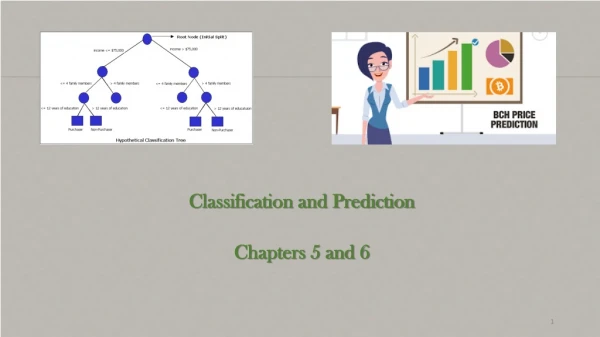
Chapter 6. Classification and Prediction
What is classification? What is prediction? Issues regarding classification and prediction Classification by decision tree induction Bayesian classification Rule-based classification Classification by back propagation. Support Vector Machines (SVM) Associative classification

Chapter 6. Classification and Prediction
E N D
Presentation Transcript
What is classification? What is prediction? Issues regarding classification and prediction Classification by decision tree induction Bayesian classification Rule-based classification Classification by back propagation Support Vector Machines (SVM) Associative classification Lazy learners (or learning from your neighbors) Other classification methods Prediction Accuracy and error measures Ensemble methods Model selection Summary Chapter 6. Classification and Prediction Data Mining: Concepts and Techniques
Classification vs. Prediction • Classification • predicts categorical class labels (discrete or nominal) • classifies data (constructs a model) based on the training set and the values (class labels) in a classifying attribute and uses it in classifying new data • Prediction • models continuous-valued functions, i.e., predicts unknown or missing values • Typical applications • Credit approval • Target marketing • Medical diagnosis • Fraud detection Data Mining: Concepts and Techniques
Classification—A Two-Step Process • Model construction: describing a set of predetermined classes • Each tuple/sample is assumed to belong to a predefined class, as determined by the class label attribute • The set of tuples used for model construction is training set • The model is represented as classification rules, decision trees, or mathematical formulae • Model usage: for classifying future or unknown objects • Estimate accuracy of the model • The known label of test sample is compared with the classified result from the model • Accuracy rate is the percentage of test set samples that are correctly classified by the model • Test set is independent of training set, otherwise over-fitting will occur • If the accuracy is acceptable, use the model to classify data tuples whose class labels are not known Data Mining: Concepts and Techniques
Training Data Classifier (Model) Process (1): Model Construction Classification Algorithms IF rank = ‘professor’ OR years > 6 THEN tenured = ‘yes’ Data Mining: Concepts and Techniques
Classifier Testing Data Unseen Data Process (2): Using the Model in Prediction (Jeff, Professor, 4) Tenured? Data Mining: Concepts and Techniques
Supervised vs. Unsupervised Learning • Supervised learning (classification) • Supervision: The training data (observations, measurements, etc.) are accompanied by labels indicating the class of the observations • New data is classified based on the training set • Unsupervised learning(clustering) • The class labels of training data is unknown • Given a set of measurements, observations, etc. with the aim of establishing the existence of classes or clusters in the data Data Mining: Concepts and Techniques
What is classification? What is prediction? Issues regarding classification and prediction Classification by decision tree induction Bayesian classification Rule-based classification Classification by back propagation Support Vector Machines (SVM) Associative classification Lazy learners (or learning from your neighbors) Other classification methods Prediction Accuracy and error measures Ensemble methods Model selection Summary Chapter 6. Classification and Prediction Data Mining: Concepts and Techniques
Issues: Data Preparation • Data cleaning • Preprocess data in order to reduce noise and handle missing values • Relevance analysis (feature selection) • Remove the irrelevant or redundant attributes • Data transformation • Generalize and/or normalize data Data Mining: Concepts and Techniques
Issues: Evaluating Classification Methods • Accuracy • classifier accuracy: predicting class label • predictor accuracy: guessing value of predicted attributes • Speed • time to construct the model (training time) • time to use the model (classification/prediction time) • Robustness: handling noise and missing values • Scalability: efficiency in disk-resident databases • Interpretability • understanding and insight provided by the model • Other measures, e.g., goodness of rules, such as decision tree size or compactness of classification rules Data Mining: Concepts and Techniques
What is classification? What is prediction? Issues regarding classification and prediction Classification by decision tree induction Bayesian classification Rule-based classification Classification by back propagation Support Vector Machines (SVM) Associative classification Lazy learners (or learning from your neighbors) Other classification methods Prediction Accuracy and error measures Ensemble methods Model selection Summary Chapter 6. Classification and Prediction Data Mining: Concepts and Techniques
Decision Tree Induction: Training Dataset This follows an example of Quinlan’s ID3 (Playing Tennis) Data Mining: Concepts and Techniques
age? <=30 overcast >40 31..40 student? credit rating? yes excellent fair no yes no yes no yes Output: A Decision Tree for “buys_computer” Data Mining: Concepts and Techniques
Algorithm for Decision Tree Induction • Basic algorithm (a greedy algorithm) • Tree is constructed in a top-down recursive divide-and-conquer manner • At start, all the training examples are at the root • Attributes are categorical (if continuous-valued, they are discretized in advance) • Examples are partitioned recursively based on selected attributes • Test attributes are selected on the basis of a heuristic or statistical measure (e.g., information gain) • Conditions for stopping partitioning • All samples for a given node belong to the same class • There are no remaining attributes for further partitioning – majority voting is employed for classifying the leaf • There are no samples left Data Mining: Concepts and Techniques
Attribute Selection Measure: Information Gain (ID3/C4.5) • Select the attribute with the highest information gain • Let pi be the probability that an arbitrary tuple in D belongs to class Ci, estimated by |Ci, D|/|D| • Expected information (entropy) needed to classify a tuple in D: • Information needed (after using A to split D into v partitions) to classify D: • Information gained by branching on attribute A Data Mining: Concepts and Techniques
Class P: buys_computer = “yes” Class N: buys_computer = “no” means “age <=30” has 5 out of 14 samples, with 2 yes’es and 3 no’s. Hence Similarly, Attribute Selection: Information Gain Data Mining: Concepts and Techniques
Computing Information-Gain for Continuous-Value Attributes • Let attribute A be a continuous-valued attribute • Must determine the best split point for A • Sort the value A in increasing order • Typically, the midpoint between each pair of adjacent values is considered as a possible split point • (ai+ai+1)/2 is the midpoint between the values of ai and ai+1 • The point with the minimum expected information requirement for A is selected as the split-point for A • Split: • D1 is the set of tuples in D satisfying A ≤ split-point, and D2 is the set of tuples in D satisfying A > split-point Data Mining: Concepts and Techniques
Gain Ratio for Attribute Selection (C4.5) • Information gain measure is biased towards attributes with a large number of values • C4.5 (a successor of ID3) uses gain ratio to overcome the problem (normalization to information gain) • GainRatio(A) = Gain(A)/SplitInfo(A) • Ex. • gain_ratio(income) = 0.029/0.926 = 0.031 • The attribute with the maximum gain ratio is selected as the splitting attribute Data Mining: Concepts and Techniques
Gini index (CART, IBM IntelligentMiner) • If a data set D contains examples from n classes, gini index, gini(D) is defined as where pj is the relative frequency of class j in D • If a data set D is split on A into two subsets D1 and D2, the gini index gini(D) is defined as • Reduction in Impurity: • The attribute provides the smallest ginisplit(D) (or the largest reduction in impurity) is chosen to split the node (need to enumerate all the possible splitting points for each attribute) Data Mining: Concepts and Techniques
Gini index (CART, IBM IntelligentMiner) • Ex. D has 9 tuples in buys_computer = “yes” and 5 in “no” • Suppose the attribute income partitions D into 10 in D1: {low, medium} and 4 in D2 but gini{medium,high} is 0.30 and thus the best since it is the lowest • All attributes are assumed continuous-valued • May need other tools, e.g., clustering, to get the possible split values • Can be modified for categorical attributes Data Mining: Concepts and Techniques
Comparing Attribute Selection Measures • The three measures, in general, return good results but • Information gain: • biased towards multivalued attributes • Gain ratio: • tends to prefer unbalanced splits in which one partition is much smaller than the others • Gini index: • biased to multivalued attributes • has difficulty when # of classes is large • tends to favor tests that result in equal-sized partitions and purity in both partitions Data Mining: Concepts and Techniques
Comparison among Splitting Criteria For a 2-class problem: t is a node and we have c (=2, here) different class labels, p is the probability of class 1. Entropy(t)= Gini(t)=1- Classification error(t)=
Other Attribute Selection Measures • CHAID: a popular decision tree algorithm, measure based on χ2 test for independence • C-SEP: performs better than info. gain and gini index in certain cases • G-statistics: has a close approximation to χ2 distribution • MDL (Minimal Description Length) principle (i.e., the simplest solution is preferred): • The best tree as the one that requires the fewest # of bits to both (1) encode the tree, and (2) encode the exceptions to the tree • Multivariate splits (partition based on multiple variable combinations) • CART: finds multivariate splits based on a linear comb. of attrs. • Which attribute selection measure is the best? • Most give good results, none is significantly superior than others Data Mining: Concepts and Techniques
Overfitting and Tree Pruning • Overfitting: An induced tree may overfit the training data • Too many branches, some may reflect anomalies due to noise or outliers • Poor accuracy for unseen samples • Two approaches to avoid overfitting • Prepruning: Halt tree construction early—do not split a node if this would result in the goodness measure falling below a threshold • Difficult to choose an appropriate threshold • Postpruning: Remove branches from a “fully grown” tree—get a sequence of progressively pruned trees • Use a set of data different from the training data to decide which is the “best pruned tree” Data Mining: Concepts and Techniques
Enhancements to Basic Decision Tree Induction • Allow for continuous-valued attributes • Dynamically define new discrete-valued attributes that partition the continuous attribute value into a discrete set of intervals • Handle missing attribute values • Assign the most common value of the attribute • Assign probability to each of the possible values • Attribute construction • Create new attributes based on existing ones that are sparsely represented • This reduces fragmentation, repetition, and replication Data Mining: Concepts and Techniques
What is classification? What is prediction? Issues regarding classification and prediction Classification by decision tree induction Bayesian classification Rule-based classification Classification by back propagation Support Vector Machines (SVM) Associative classification Lazy learners (or learning from your neighbors) Other classification methods Prediction Accuracy and error measures Ensemble methods Model selection Summary Chapter 6. Classification and Prediction Data Mining: Concepts and Techniques
Bayesian Classification: Why? • A statistical classifier: performs probabilistic prediction, i.e., predicts class membership probabilities • Foundation: Based on Bayes’ Theorem. • Performance: A simple Bayesian classifier, naïve Bayesian classifier, has comparable performance with decision tree and selected neural network classifiers • Incremental: Each training example can incrementally increase/decrease the probability that a hypothesis is correct — prior knowledge can be combined with observed data • Standard: Even when Bayesian methods are computationally intractable, they can provide a standard of optimal decision making against which other methods can be measured Data Mining: Concepts and Techniques
Bayesian Theorem: Basics • Let X be a data sample (“evidence”): class label is unknown • Let H be a hypothesis that X belongs to class C • Classification is to determine P(H|X), the probability that the hypothesis holds given the observed data sample X • P(H) (prior probability), the initial probability • E.g., X will buy computer, regardless of age, income, … • P(X): probability that sample data is observed • P(X|H) (posteriori probability), the probability of observing the sample X, given that the hypothesis holds • E.g.,Given that X will buy computer, the prob. that X is 31..40, medium income Data Mining: Concepts and Techniques
Bayesian Theorem • Given training dataX, posteriori probability of a hypothesis H, P(H|X), follows the Bayes theorem • Informally, this can be written as posteriori = likelihood x prior/evidence • Predicts X belongs to C2 iff the probability P(Ci|X) is the highest among all the P(Ck|X) for all the k classes • Practical difficulty: require initial knowledge of many probabilities, significant computational cost Data Mining: Concepts and Techniques
Towards Naïve Bayesian Classifier • Let D be a training set of tuples and their associated class labels, and each tuple is represented by an n-D attribute vector X = (x1, x2, …, xn) • Suppose there are m classes C1, C2, …, Cm. • Classification is to derive the maximum posteriori, i.e., the maximal P(Ci|X) • This can be derived from Bayes’ theorem • Since P(X) is constant for all classes, only needs to be maximized Data Mining: Concepts and Techniques
Derivation of Naïve Bayes Classifier • A simplified assumption: attributes are conditionally independent (i.e., no dependence relation between attributes): • This greatly reduces the computation cost: Only counts the class distribution • If Ak is categorical, P(xk|Ci) is the # of tuples in Ci having value xk for Ak divided by |Ci, D| (# of tuples of Ci in D) • If Ak is continous-valued, P(xk|Ci) is usually computed based on Gaussian distribution with a mean μ and standard deviation σ and P(xk|Ci) is Data Mining: Concepts and Techniques
Naïve Bayesian Classifier: Training Dataset Class: C1:buys_computer = ‘yes’ C2:buys_computer = ‘no’ Data sample X = (age <=30, Income = medium, Student = yes Credit_rating = Fair) Data Mining: Concepts and Techniques
Naïve Bayesian Classifier: An Example • P(Ci): P(buys_computer = “yes”) = 9/14 = 0.643 P(buys_computer = “no”) = 5/14= 0.357 • Compute P(X|Ci) for each class P(age = “<=30” | buys_computer = “yes”) = 2/9 = 0.222 P(age = “<= 30” | buys_computer = “no”) = 3/5 = 0.6 P(income = “medium” | buys_computer = “yes”) = 4/9 = 0.444 P(income = “medium” | buys_computer = “no”) = 2/5 = 0.4 P(student = “yes” | buys_computer = “yes) = 6/9 = 0.667 P(student = “yes” | buys_computer = “no”) = 1/5 = 0.2 P(credit_rating = “fair” | buys_computer = “yes”) = 6/9 = 0.667 P(credit_rating = “fair” | buys_computer = “no”) = 2/5 = 0.4 • X = (age <= 30 , income = medium, student = yes, credit_rating = fair) P(X|Ci) : P(X|buys_computer = “yes”) = 0.222 x 0.444 x 0.667 x 0.667 = 0.044 P(X|buys_computer = “no”) = 0.6 x 0.4 x 0.2 x 0.4 = 0.019 P(X|Ci)*P(Ci) : P(X|buys_computer = “yes”) * P(buys_computer = “yes”) = 0.028 P(X|buys_computer = “no”) * P(buys_computer = “no”) = 0.007 Therefore, X belongs to class (“buys_computer = yes”) Data Mining: Concepts and Techniques
Avoiding the 0-Probability Problem • Naïve Bayesian prediction requires each conditional prob. be non-zero. Otherwise, the predicted prob. will be zero • Ex. Suppose a dataset with 1000 tuples, income=low (0), income= medium (990), and income = high (10), • Use Laplacian correction (or Laplacian estimator) • Adding 1 to each case Prob(income = low) = 1/1003 Prob(income = medium) = 991/1003 Prob(income = high) = 11/1003 • The “corrected” prob. estimates are close to their “uncorrected” counterparts Data Mining: Concepts and Techniques
Naïve Bayesian Classifier: Comments • Advantages • Easy to implement • Good results obtained in most of the cases • Disadvantages • Assumption: class conditional independence, therefore loss of accuracy • Practically, dependencies exist among variables • E.g., hospitals: patients: Profile: age, family history, etc. Symptoms: fever, cough etc., Disease: lung cancer, diabetes, etc. • Dependencies among these cannot be modeled by Naïve Bayesian Classifier • How to deal with these dependencies? • Bayesian Belief Networks Data Mining: Concepts and Techniques
Y Z P Bayesian Belief Networks • Bayesian belief network allows a subset of the variables conditionally independent • A graphical model of causal relationships • Represents dependency among the variables • Gives a specification of joint probability distribution • Nodes: random variables • Links: dependency • X and Y are the parents of Z, and Y is the parent of P • No dependency between Z and P • Has no loops or cycles X Data Mining: Concepts and Techniques
(FH, S) (FH, ~S) (~FH, S) (~FH, ~S) LC 0.8 0.7 0.5 0.1 ~LC 0.2 0.5 0.3 0.9 Bayesian Belief Network: An Example Family History Smoker The conditional probability table (CPT) for variable LungCancer: LungCancer Emphysema CPT shows the conditional probability for each possible combination of its parents PositiveXRay Dyspnea Derivation of the probability of a particular combination of values of X, from CPT: Bayesian Belief Networks Data Mining: Concepts and Techniques
Training Bayesian Networks • Several scenarios: • Given both the network structure and all variables observable: learn only the CPTs • Network structure known, some hidden variables: gradient descent (greedy hill-climbing) method, analogous to neural network learning • Network structure unknown, all variables observable: search through the model space to reconstruct network topology • Unknown structure, all hidden variables: No good algorithms known for this purpose • Ref. D. Heckerman: Bayesian networks for data mining Data Mining: Concepts and Techniques
What is classification? What is prediction? Issues regarding classification and prediction Classification by decision tree induction Bayesian classification Rule-based classification Classification by back propagation Support Vector Machines (SVM) Associative classification Lazy learners (or learning from your neighbors) Other classification methods Prediction Accuracy and error measures Ensemble methods Model selection Summary Chapter 6. Classification and Prediction Data Mining: Concepts and Techniques
Neural Network as a Classifier • Weakness • Long training time • Require a number of parameters typically best determined empirically, e.g., the network topology or ``structure." • Poor interpretability: Difficult to interpret the symbolic meaning behind the learned weights and of ``hidden units" in the network • Strength • High tolerance to noisy data • Ability to classify untrained patterns • Well-suited for continuous-valued inputs and outputs • Successful on a wide array of real-world data • Algorithms are inherently parallel • Techniques have recently been developed for the extraction of rules from trained neural networks Data Mining: Concepts and Techniques
Classification by Backpropagation • Backpropagation: A neural network learning algorithm • Started by psychologists and neurobiologists to develop and test computational analogues of neurons • A neural network: A set of connected input/output units where each connection has a weight associated with it • During the learning phase, the network learns by adjusting the weights so as to be able to predict the correct class label of the input tuples • Also referred to as connectionist learning due to the connections between units Data Mining: Concepts and Techniques
- mk x0 w0 x1 w1 f å output y xn wn Input vector x weight vector w weighted sum Activation function A Neuron (= a perceptron) • The n-dimensional input vector x is mapped into variable y by means of the scalar product and a nonlinear function mapping Data Mining: Concepts and Techniques
Network Training • The ultimate objective of training • obtain a set of weights that makes almost all the tuples in the training data classified correctly • Steps • Initialize weights with random values • Feed the input tuples into the network one by one • For each unit • Compute the net input to the unit as a linear combination of all the inputs to the unit • Compute the output value using the activation function • Compute the error • Update the weights and the bias
Multi-Layer Perceptron Output vector Output nodes Hidden nodes wij Input nodes Input vector: xi
Gradient Descent Rule Data Mining: Concepts and Techniques
The vector derivative called the gradient of E with respect to w is written E(w). • The gradient specifies the direction that produces the steepest increase in E. • Thenegative of this vector gives the direction of steepest decrease. Data Mining: Concepts and Techniques
The training rule for gradient descent is • where • For component wi , • wiwi + wi, and wi= • In short, the steepest descent is achieved by altering each component wi of w in proportion to Data Mining: Concepts and Techniques
is a positive constant called the learning rate, which determines the step size in the gradient descent search. • Usually, the error function Ed(w) for each individual training example d is defined as follows Data Mining: Concepts and Techniques
Backpropagation rule • Updating weight wji by adding to it wji, for training example d. • Ed is the error on training example d, summed over all output units in the network. • Outputs is the set of output units in the network, tk is the target value of unit k for training example d, and ok is the output of unit k given training example d. Data Mining: Concepts and Techniques