Download
1 / 37
370 likes | 480 Views
GLOBAL CHANGE AND AIR POLLUTION (GCAP):. Work to date and future plans. an EPA-STAR project. Daniel J. Jacob (P.I.) and Loretta J. Mickley, Harvard John H. Seinfeld, Caltech David Rind, NASA/GISS Joshua Fu, U. Tennessee David G. Streets, ANL Daewon Byun, U. Houston. 2000-2050 change in

E N D
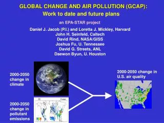
GLOBAL CHANGE AND AIR POLLUTION (GCAP): Work to date and future plans an EPA-STAR project Daniel J. Jacob (P.I.) and Loretta J. Mickley, Harvard John H. Seinfeld, Caltech David Rind, NASA/GISS Joshua Fu, U. Tennessee David G. Streets, ANL Daewon Byun, U. Houston 2000-2050 change in U.S. air quality 2000-2050 change in climate 2000-2050 change in pollutant emissions
THE GCAP STRATEGY IPCC scenarios and derived emissions ozone and PM precursors mercury greenhouse gases boundary conditions met. input GEOS-Chem CTM global O3-PM-Hg simulation GISS GCM 3 1950-2050 transient climate simulation CMAQ O3-PM-Hg simulation 2050 vs. 2000 climate MM5 mesoscale dynamics simulation boundary conditions met. input
GCAP WORK TO DATE • Analysis of 2000-2050 trends in air pollution meteorology • Development of GISS/GEOS-Chem interface • Development of GISS/MM5 interface • Development of future emission inventories for carbonaceous aerosols • Application of GISS/GEOS-Chem to 2000-2050 trends in ozone and PM (IPCC A1 scenario) • Statistical projection of 2000-2100 ozone trends
Clean air sweeps behind cold front GISS GCM 2’ simulations for 2050 vs. present-day climate using pollution tracers with constant emissions Mid-latitudes cyclones tracking across southern Canada are the main drivers of northern U.S. ventilation EFFECT OF CLIMATE CHANGE ON REGIONAL STAGNATION Sunday night’s weather map 2045-2052 Northeast U.S. CO pollution tracer summer 1995-2002 Pollution episodes double in duration in 2050 climate due to decreasing frequency of cyclones ventilating the eastern U.S; this decrease is an expected consequence of greenhouse warming. Mickley et al. [2004]
CLIMATOLOGICAL DATA SHOW DECREASE IN FREQUENCY OF MID-LATITUDE CYCLONESOVER PAST 50 YEARS 1000 Annual number of surface cyclones and anticylones over North America cyclones 500 Agee [1991] 100 anticyclones 1980 1950 Cyclone frequency at 30o-60oN McCabe et al. [2001]
NH winter N. America summer GCM vs. OBSERVED 1950-2000 TRENDS IN CYCLONE FREQUENCIES 40% simulated decrease in cyclone frequency for N. America for 1950-2000, consistent with observations Eric M. Leibensperger, Harvard
REDUCED VENTILATION OF CENTRAL/EASTERN U.S. IN FUTURE CLIMATE DU TO LOWER CYCLONE FREQUENCY Summertime cyclone tracks for three years of GISS GCM climate show 14 % decrease in number of cyclones as well as a poleward shift. 2000 climate 2050 climate 2049-2051 1999-2001 Consistent with IPCC [2007] analysis of output from 20 GCMs [Lambert et al., 2006] Eric M. Leibensperger, Harvard
DRIVING GEOS-Chem WITH GISS GCM 3 OUTPUT 6-hour archive: winds, convective mass fluxes, temperature, humidity, cloud optical depths, precipitation… 3-hour archive: mixing depths, surface properties replicates structure of NASA/GEOS assimilated data archive (0.5ox0.625o) used to drive standard GEOS-Chem GEOS-Chem O3-PM-Hg simulation 4ox5o, 23L GISS GCM 3 transient climate simulation 4ox5o, 23L Option of using GISS GCM met. fields is now part of the standard GEOS-Chem Wu et al. [2007a]
Present-climate simulation (3 yrs) vs. GEOS-3 (2001), GEOS-4 (2001). ozonesondes EVALUATION OF GISS/GEOS-Chem OZONE SIMULATION GISS (3 yrs) GEOS-3 Global ozone budgets: GEOS-4 July surface afternoon ozone (ppbv) Wu et al. [2007a]
Evaluation of Present-day Sulfate: Measurements Averaged over 2001-2003 GISS/GEOS-Chem IMPROVE Simulated vs. IMPROVE Annual Mean Conc. Simulated vs. NADP Annual Mean Wet Deposition R=0.95 S=0.73 R=0.86 S=1.0 Liao et al. [2007]
Evaluation of Present-day Nitrate, BC, and OC GCAP IMPROVE Simulated vs. IMPROVE R=0.35 S=0.91 R=0.67 S=0.98 R=0.72 S=0.77 R=0.41 S=0.60 Annual Mean Nitrate Annual Mean BC Seasonal Mean OC DJF Seasonal Mean OC JJA Liao et al. [2007]
SIMULATED vs. OBSERVED PM2.5 AT IMPROVE SITES Annual mean 2001-2003 values simulated observed correlation R = 0.84 S = 0.77 SOA/PM2.5 up to 60% in NW 10-20% in SE 50% of simulated SOA Is from isoprene Liao et al. [2007]
2000 emissions: GEOS-Chem, including NEI 99 for United States 2000-2050 % change, anthropogenic: SRES A1B scenario 2000-2050 % change, natural: GISS/GEOS-Chem 2000-2050 CHANGES IN EMISSIONS OF OZONE PRECURSORS Wu et al. [2007b]
2000 concentrations (ppb) 2050 climate / 2000 2050 emissions / 2000 2050 / 2000 Climate change increases global tropospheric ozone (mostly from lightning) but generally decreases surface ozone (mostly because of water vapor) 2000-2050 CHANGE IN GLOBAL TROPOSPHERIC OZONE +3% +20% +17% Wu et al. [2007b]
2050 climate decreases PRB in subsiding regions, increases in upwelling regions 2050 emissions increases PRB due to rising methane, Asian emissions The two effects cancel in the eastern U.S. CHANGE IN POLICY-RELEVANT BACKGROUND (PRB) OZONE 1999-2001 PRB ozone (ppb) D (2000 emissions & 2050 climate) D (2050 emissions & 2000 climate) D (2050 emissions & climate) Wu et al. [2007b]
EFFECTS OF 2000-2050 CHANGES IN CLIMATE AND GLOBALEMISSIONSON MEAN 8-h AVG. DAILY MAXMUM OZONE IN SUMMER 1999-2001 ozone, ppb D (2000 emissions w/ 2050 climate) D (2050 emissions & 2000 climate) D (2050 emissions & climate) Wu et al. [2007b]
METEOROLOGICAL FACTORS DRIVING 2000-2050 CLIMATE CHANGE SENSITIVITY Summer afternoon differences in mean values for 2050 vs. 2000 climates 850 hPa convective flux Temperature (K) Mixing depth (2050/2000 ratio) (2050/2000 ratio) ( Mixing depths may decrease in a warmer greenhouse climate depending on soil moisture, vertical distribution of greenhouse heating Wu et al. [2007b]
Summer probability distribution of daily 8-h max ozone SENSITIVITY OF POLLUTION EPISODES TO GLOBAL CHANGE 99th 90th median • In northeast and midwest, climate change effect reaches 10 ppbv for high-O3 • events; longer and more frequent stagnation episodes • near-zero effect In southeast Wu et al. [2007b]
WHAT IS THE CLIMATE CHANGE PENALTY IN TERMS OF ADDED REQUIREMENTS ON EMISSION REDUCTIONS? 2000 climate with NOx emissions reduced by 40% 2050 climate - 50% NOx 2050 climate - 60% NOx 2000-2050 climate change means that we will need to reduce NOx emissions by 50% instead of 40% to achieve the same ozone air quality goals in the northeast Wu et al. [2007b]
OZONE CLIMATE CHANGE PENALTY WILL BE HIGHER IF WE DON’T REDUCE EMISSIONS Change in mean 8-h daily max ozone (ppb) from 2000-2050 climate change with 2000 emissions with 2050 emissions Reducing U.S. anthropogenic emissions significantly mitigates the climate change penalty Wu et al. [2007b]
2000-2050 EMISSIONS OF PM2.5 PRECURSORS (A1) David Streets, ANL and Shiliang Wu, Harvard
OC/Energy BC/Energy OC/Biomass BC/Biomass CONSTRUCTION OF SRES-BASED EMISSION PROJECTIONSFOR BC AND OC AEROSOL Global and U.S. decreases in emissions (higher energy efficiency) Streets et al. [2004]
EFFECT OF 2000-2050 GLOBAL CHANGE ON ANNUAL MEAN SULFATE CONCENTRATIONS (mg m-3) Climate change increases sulfate by up to 0.5 mg m-3 in midwest (more stagnation), decreases sulfate in southeast (more precipitation) 2000 conditions: sulfate, mg m-3D(2000 emissions & 2050 climate) D (2050 emissions & 2000 climate) D 2050 emissions & 2050 climate) Shiliang Wu, Harvard
EFFECT OF 2000-2050 GLOBAL CHANGE ON ANNUAL MEAN NITRATE CONCENTRATIONS (mg m-3) Climate change decreases nitrate by up to 0.2 mg m-3 (higher temperature) 1999-2001 nitrate (mg m-3) D (2000 emissions & 2050 climate) D (2050 emissions & 2000 climate D (2050 emissions & climate) Shiliang Wu, Harvard
EFFECT OF 2000-2050 GLOBAL CHANGE ON ANNUAL MEAN BC AEROSOL CONCENTRATIONS (mg m-3) Climate change increases BC by up to 0.05 mg C m-3 in northeast 1999-2001 BC (mg m-3) D (2000 emissions & 2050 climate) D (2050 emissions & 2000 climate) D (2050 emissions & climate) Shiliang Wu, Harvard
EFFECT OF 2000-2050 GLOBAL CHANGE ON ANNUAL MEAN ORGANIC CARBON (OC) AEROSOL CONCENTRATIONS (mg m-3) Climate change effect is mainly through biogenic SOA and is small because of compensating factors (higher biogenic VOCs, higher volatility) Expect larger effects from increases in wildfires (not included here) 2000 conditions: OC, mg m-3D(2000 emissions & 2050 climate) D (2050 emissions & 2000 climate) D 2050 emissions & 2050 climate) Shiliang Wu, Harvard
2000 conditions: PM2.5, mg m-3D(2000 emissions & 2050 climate) D (2050 emissions & 2000 climate) D 2050 emissions & 2050 climate) EFFECT OF 2000-2050 GLOBAL CHANGE ON ANNUAL MEAN PM2.5 CONCENTRATIONS (mg m-3) Effect of climate change is positive but small (at most 0.3 mg m-3), due to canceling effects Shiliang Wu, Harvard
Surface air density NCEP/MM5 GISS/MM5 test application for East Asia INTERFACING GISS/GEOS-Chem WITH MM5/CMAQ Driving MM5 with GISS vs. NCEP: interface is completed, being tested Driving CMAQ with GEOS-Chem BCs: interface is mature surface ozone surface PM2.5 Joshua Fu, UT
DETERMINISTIC vs. STATISTICAL MODELING APPROACHES FOR DIAGNOSING EFFECT OF CLIMATE CHANGE ON AIR QUALITY DETERMINISTIC STATISTICAL GCM D global climate Global CTM RCM statistical downscaling D regional climate D global chemistry • air quality = f(D meteorology) local statistical model Regional CTM D air quality
# summer days with 8-hour O3 > 84 ppbv, average for northeast U.S. sites 1988, hottest on record USE OBSERVED OZONE-TEMPERATURE RELATIONSHIP TO DIAGNOSE SENSITIVITY OF OZONE TO CLIMATE CHANGE Observed relationship of ozone vs. T characterizes the total derivative: where xi is the ensemble of T-dependent variables affecting ozone; … and can diagnose effect of climate change as characterized by DT from a GCM Northeast Los Angeles Southeast Probability of max 8-h O3 > 84 ppbv vs. daily max. T Lin et al. [2001]
STATISTICAL METHOD TO PROJECT NAAQS EXCEEDANCESFOR A GIVEN LOCATION OR REGION IN A FUTURE CLIMATE Apply ensemble of GCMs to simulate future climate Obtain daily max T for individual grid squares Apply subgrid variability to T from present-day climatology Obtain daily max T for individual locations Apply local or regional probability of NAAQS exceedance = f(T) Obtain probability of NAAQS exceedance in future climate assuming constant emissions
APPLICATION TO PROJECT FUTURE EXCEEDANCES OF OZONE NAAQSIN THE NORTHEAST UNITED STATES Three IPCC(2007) GCMs, downscaled to capture local variability Northeast U.S. • Statistical method allows quick local assessment of the effect of climate change, • but it has limitations: • gives no insight into the coupled effect of changing emissions • some fraction of variance unresolved by statistical model • no good statistical relationships for PM developed so far Loretta Mickley (Harvard) and Cynthia Lin (UC Davis)
GCAP FUTURE PLANS • Downscale GEOS-Chem future-climate simulations to CMAQ • Improve GCM (GISS)- RCM (MM5) meteorological interface • Apply additional scenarios for global change in climate and emissions • Diagnose intercontinental transport in the future atmosphere • Study effects of 2000-2050 climate and emission changes on mercury, including construction of future mercury emission inventories • Explore correlations of PM2.5 with meteorological variables for future-climate statistical projections
RAPIDLY CHANGING ANTHROPOGENIC EMISSIONS OF MERCURY:recent shift from N.America/Europe to Asia 1990 Total: 1.88 Gg yr-1 2000 Total: 2.27 Gg yr-1 Pacyna and Pacyna, 2005
GEOS-Chem SIMULATION OF TOTAL GASEOUS MERCURY (TGM) Annual mean surface air concentrations and ship cruise data Circles are observations; background is model Land-based sites observed: 1.58 ± 0.19 ng m-3 model: 1.60 ± 0.10 ng m-3 Large underestimate of NH cruise data: legacy of past emissions stored in ocean? R2=0.51 Selin et al., 2007
Hg DEPOSITION OVER U.S. : LOCAL VS. GLOBAL SOURCES Wet deposition fluxes, 2003-2004 Model: contours Obs: dots max in southeast U.S. from oxidation of global Hg pool 2nd max in midwest from regional sources (mostly dry deposition in GEOS-Chem) 2/3 of Hg deposition over U.S. in model is dry, not wet! Simulated % contribution of North American sources to total Hg deposition U.S. mean: 20% Selin et al. [2007]
GEOS-Chem GLOBAL GEOCHEMICAL CYCLE OF MERCURY (present);exchanges with ocean and land are climate-dependent ATMOSPHERE; lifetime 0.8 y 5.4 0.5 2.2 2.8 1.5 3.8 3.2 evasion evasion wet &dry deposition LAND SURFACE SURFACE OCEAN 10 2.3 rivers SOIL 1000 0.2 0.6 DEEP OCEAN 280 Natural (rocks, volcanoes) Anthropogenic (fossil fuels) burial 0.5 uplift SEDIMENTS Selin et al. [2007], Strode et al. [2007] Inventories in Gg, fluxes in Gg yr-1