Exploring Relationships: Scatterplots & Correlation
230 likes | 251 Views
Understand scatterplots, outliers, and correlation in bivariate data analysis. Learn how to interpret graphical displays and numerical summaries to identify patterns and deviations. Explore the impact of different variables on each other.

Exploring Relationships: Scatterplots & Correlation
E N D
Presentation Transcript
Scatterplot Objectives • Scatterplots • Explanatory and response variables • Interpreting scatterplots • Outliers • Categorical variables in scatterplots
Basic Terminology • Univariate data: 1 variable is measured on each sample unit or population unit (lecture unit 2) e.g. height of each student in a sample • Bivariate data: 2 variables are measured on each sample unit or population unit e.g. height and GPA of each student in a sample;(caution: data from 2 separate samples is not bivariate data)
Basic Terminology (cont.) • Multivariate data: several variables are measured on each unit in a sample or population. • For each student in a sample of NCSU students, measure height, GPA, and distance between NCSU and hometown; • Focus on bivariate data in Chapter 12
Same goals with bivariate data that we had with univariate data • Graphical displays and numerical summaries • Seek overall patterns and deviations from those patterns • Descriptive measures of specific aspects of the data
Here, we have two quantitative variables for each of 16 students. • 1) How many beers they drank, and • 2) Their blood alcohol level (BAC) • We are interested in the relationship between the two variables: How is one affected by changes in the other one?
Scatterplots • Useful method to graphically describe the relationship between 2 quantitative variables
Scatterplot: Blood Alcohol Content vs Number of Beers In a scatterplot, one axis is used to represent each of the variables, and the data are plotted as points on the graph.
Focus on Three Features of a Scatterplot Look for an overall pattern regarding … • Shape - ? Approximately linear, curved, up-and-down? • Direction - ? Positive, negative, none? • Strength - ? Are the points tightly clustered in the particular shape, or are they spread out? … and deviations from the overall pattern: Outliers
Scatterplot: Fuel Consumption vs Car Weight. x=car weight, y=fuel cons. • (xi, yi): (3.4, 5.5) (3.8, 5.9) (4.1, 6.5) (2.2, 3.3) (2.6, 3.6) (2.9, 4.6) (2, 2.9) (2.7, 3.6) (1.9, 3.1) (3.4, 4.9)
Response (dependent) variable: blood alcohol content y x Explanatory (independent) variable: number of beers Explanatory and response variables A response variablemeasures or records an outcome of a study. An explanatory variableexplains changes in the response variable. Typically, the explanatory or independent variable is plotted on the x axis, and the response or dependent variable is plotted on the y axis.
SAT Score vs Proportion of Seniors Taking SAT 2005 IW IL NC 74% 1010
Correlation Objectives • The correlation coefficient “r” • r does not distinguish x and y • r has no units • r ranges from -1 to +1 • Influential points
The correlation coefficient "r" The correlation coefficient is a measure of the direction and strength of the linear relationship between 2 quantitative variables. It is calculated using the mean and the standard deviation of both the x and y variables. Correlation can only be used to describe quantitative variables. Categorical variables don’t have means and standard deviations.
Example: calculating correlation • (x1, y1), (x2, y2), (x3, y3) • (1, 3) (1.5, 6) (2.5, 8)
Properties of Correlation • r is a measure of the strength of the linear relationship between x and y. • No units [like demand elasticity in economics (-infinity, 0)] • -1 < r < 1
Properties (cont.)r ranges from-1 to+1 "r" quantifies the strength and direction of a linear relationship between 2 quantitative variables. Strength: how closely the points follow a straight line. Direction: is positive when individuals with higher X values tend to have higher values of Y.
Properties of Correlation (cont.) • r = -1 only if y = a + bx with slope b<0 • r = +1 only if y = a + bx with slope b>0 y = 1 + 2x y = 11 - x
Properties (cont.) High correlation does not imply cause and effect CARROTS: Hidden terror in the produce department at your neighborhood grocery • Everyone who ate carrots in 1920, if they are still alive, has severely wrinkled skin!!! • Everyone who ate carrots in 1865 is now dead!!! • 45 of 50 17 yr olds arrested in Raleigh for juvenile delinquency had eaten carrots in the 2 weeks prior to their arrest !!!
Properties (cont.) Cause and Effect • There is a strong positive correlation between the monetary damage caused by structural fires and the number of firemen present at the fire. (More firemen-more damage) • Improper training? Will no firemen present result in the least amount of damage?
Properties (cont.) Cause and Effect (1,2) (24,75) (1,0) (18,59) (9,9) (3,7) (5,35) (20,46) (1,0) (3,2) (22,57) • r measures the strength of the linearrelationship between x and y; it does not indicate cause and effect • correlation r = .935 x = fouls committed by player; y = points scored by same player The correlation is due to a third “lurking” variable – playing time